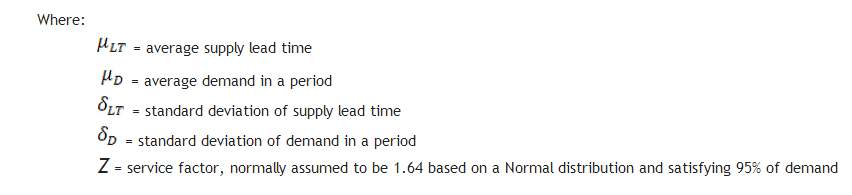
I want to take all of us down into the weeds for my next blog, "Truth, Lies, and Statistical Modeling in Supply Chain.
I came to the conclusion that this would be necessary after talking to colleagues and customers about the how we model all of our manufacturing and supply chain systems using deterministic models, when in fact everything around us is stochastic. My first clue that this was necessary was when I got a lot of puzzled looks and someone was brave enough to ask me to explain deterministic and stochastic. I came to these terms late in my education and purely through luck so I am not surprised that there is little knowledge and understanding of these terms.
Conflict #1: Most systems that run our supply chain use precise mathematical models that assume complete identification and prediction of variables (Deterministic), yet we operate in a highly unpredictable environment (Stochastic).
In essence, a deterministic approach assumes that:
- A system always operates in an entirely repeatable manner, i.e. no randomness
- We have an exact understanding of how a system works
- That we can describe the way a system works in precise mathematical equations
In contrast a stochastic approach assumes that:
- There is always some element of a system that cannot be understood and described, which exhibits itself as randomness
- We can never fully understand and describe how a system works because it is boundless
- As a consequence, systems cannot be described in precise mathematic equations
I am an engineer by training, and like most engineers I had very little exposure to statistics and probability theory until I studied Industrial Engineering and Operations Research at the graduate level. And I cannot tell you how many of my friends, studying ‘harder’ engineering courses such as Electrical or Mechanical, referred to Industrial as ‘Imaginary Engineering’ precisely because it deals in ‘fuzzy’ concepts that cannot be described fully. I stumbled into Queuing Theory by accident, which was a complete revelation to me. It is the study of the effect of randomness on serial processes, such as manufacturing and supply chain. Even in Queuing Theory most of the analysis focused on Exponential distributions because solutions are easier to derive, while using a Normal distribution makes it near impossible to derive solutions other than for very simple problems. As I have discussed previously, given my deep grounding in deterministic analysis, it took me a long time to accept some of the fundamental observations of impact on measures such as throughput and capacity utilization that result from stochastic analysis.
But it wasn’t until I started a course in Discrete Event Simulation that I was introduced to the LogNormal distribution. And this is what I want to concentrate on for this blog. My next blog will be on what this means to a supply chain planning approach based upon optimization.
Conflict #2: Many supply chain models act as if events, over time, are evenly distributed (Normal Distribution), yet most incidents and their respective magnitude (e.g. demand spikes, supply delays) are highly random (LogNormal Distribution).
Anyone who has dealt with equipment failure will be intuitively familiar with the LogNormal distribution. This is because, most of the time, failures occur after a fairly well establish mean time between failures, and every now and again the equipment fails very soon after being commissioned or repaired, but very seldom will a piece of equipment run for much longer than the mean time between failure (the Weibull distribution can also be used for failures). If the time between failures was distributed according to a Normal distribution, we would expect the time between failures to be evenly distributed around the mean, meaning it would be just as likely that the equipment would last a little longer than normal as it is to fail a little earlier than normal. But equipment failures don’t work that way. Using a Normal distribution rather than a LogNormal distribution means that we under-estimate the risk of the equipment failing early and over-estimate the risk of it failing late. There is a very good article in the Oct 2009 Harvard Business Review (HBR) titled “The Six Mistakes Executives Make in Risk Management” by Nassim N. Taleb, Daniel G. Goldstein, and Mark W. Spitznagel that addresses the consequences of assuming a Normal distribution. In a section called “We assume that risk can be measured by standard deviation”, they state that:
Standard deviation—used extensively in finance as a measure of investment risk— shouldn’t be used in risk management. The standard deviation corresponds to the square root of average squared variations—not average variations. The use of squares and square roots makes the measure complicated. It only means that, in a world of tame randomness, around two-thirds of changes should fall within certain limits (the –1 and +1 standard deviations) and that variations in excess of seven standard deviations are practically impossible. However, this is inapplicable in real life, where movements can exceed 10, 20, or sometimes even 30 standard deviations. Risk managers should avoid using methods and measures connected to standard deviation, such as regression models, R-squares, and betas.
And yet the Normal distribution and associated standard deviation measures are used in the quintessential supply chain risk management practice of Inventory Optimization. The classic inventory optimization equations all try to mitigate the risk of not having inventory to satisfy customer demand by defining a certain safety stock required to achieve a desired customer service level. Here is the rub: By assuming a Normal distribution when in fact a LogNormal distribution applies, we are in fact both underestimating the risk of running out of inventory and carrying too much inventory. For those of you who doubt that a LogNormal distribution applies to demand, just think of the number of times there is an unexpectedly large order versus an unexpectedly small order. Let’s explore the consequence to inventory optimization by starting with the distribution of demand and supply lead times, the principal variables used to calculate inventory.
Conflict #3: The more variable the elements, the less effective the standard models are (the proof is in the math!)
Starting on the demand side, the Coefficient of Variation – CoV = StdDev/Mean – is often used to measure demand variability, with CoV of below 0.25 being considered stable demand and CoV above 1.5 being considered very variable. Below is a diagram – I apologize for the quality – of example CoV for several industries. As we can see from these diagrams it is really only Consumer Packaged Goods companies – Bottled Food Product Mixes and Dry Packaged Food Products - that see demand with a CoV much below 1 for a significant portion of their items, and only a few experience items with a CoV below 0.25. These are so-called High Volume/Low Mix industries. The rest of the industries experience a significant proportion of their demand from items with a CoV greater than 1. These are Low Volume/High Mix industries.
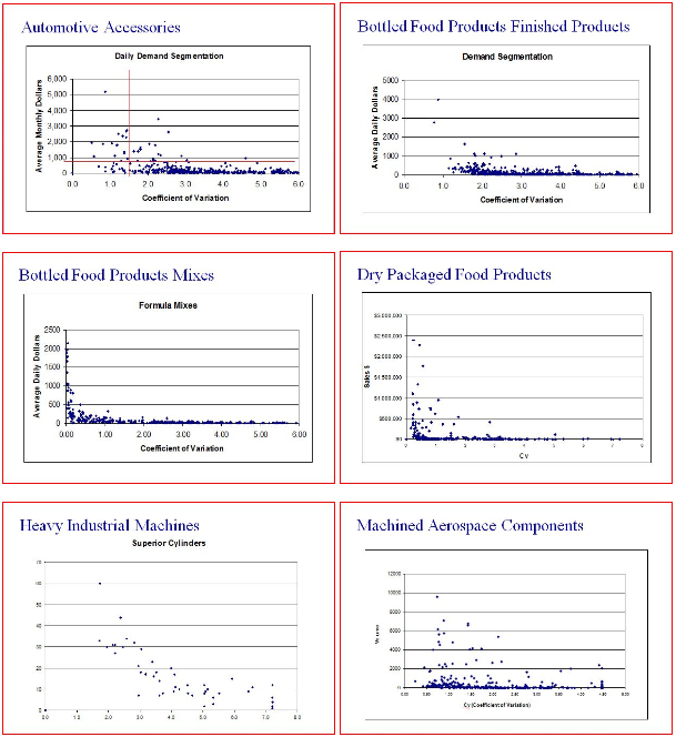
The significance of these graphs is that any demand with a CoV over 0.2 does not follow a Normal distribution. Demand with a CoV greater than 0.2 cannot be following a Normal distribution, and is most likely following a LogNormal distribution. To prove that a CoV greater than 0.2 means that demand is not Normally distributed I ran a little experiment in Excel that resulted in the following graph which measures the probability of generating negative values from a Normal distribution with a mean of 100 and different standard deviations determined by the CoV (the Excel code is at the end of the blog). For each CoV value I sampled 1,000,000 values from a Normal distribution with a mean of 100 and the standard deviation of 100*CoV, and counted the negative values generated. The probability is simply the number of negative values divided by 1,000,000.
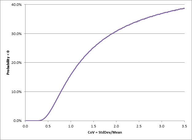
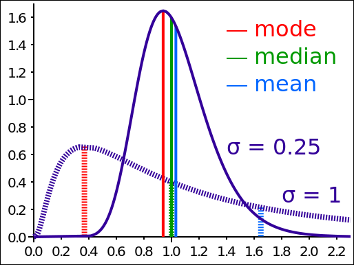
As can be seen from the diagram, there is about a 17% chance of a negative value with a CoV of 1, and nearly a 29% chance of a negative value with a CoV of 2. In other words, if we assume that demand is Normally distributed and from experience we know the CoV to be 2, then we must be experiencing negative demand nearly 1/3 of the time. So, here is my question: When last did you see a negative demand? Sure there are returns, but demand in a period isn’t going to be negative. So there must be something else driving the high variability, namely that demand does not follow a Normal distribution, and most likely it is following a LogNormal distribution. In many cases in business-to-business transactions there is a minimum purchase quantity, which very often drives purchasing behavior. But every now and then there will be a large demand spike. This is the classic behavior of LogNormal distribution. The same can be said for the supply lead time, the other input to inventory optimization calculations. Much of the time we experience lead times we expect, but never a negative lead time, and sometimes we experience long lead times. In other words very often supply lead time will also follow a LogNormal distribution. Modeling supply lead times using a Normal distribution will mean that at times we experience a negative lead time. So what does a LogNormal distribution look like? Example 1: A key point to note is that both distributions in the diagram below have a median of 1, but the mode and mean are very different. Also note that the CoV for the solid line is about 0.25 (0.25/1) whereas for the dashed line the CoV is about 0.61 (1/1.63). Neither is anywhere near the CoV of 3 experienced in some of the industries above.
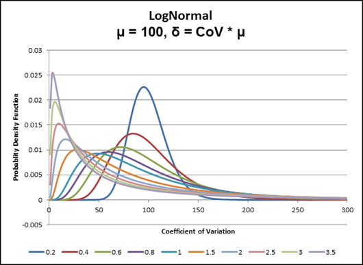
Example 2: Conversely, every LogNormal distribution in the diagram below has a mean of 100. The only difference between the curves is the CoV, or the degree of variability. The smaller the standard deviation (smaller CoV) the more the LogNormal distribution looks like a Normal or Gaussian distribution. But note that by the time the CoV is 0.4 there is a big difference. Also note that there are no negative values. Even for a CoV of 0.2 the distribution is not perfectly symmetrical about the mean, as can be seen by the fact that the curve goes to zero at about 60 on the left (40 from the mean of 100), but at about 175 on the right (75 from the mean of 100).
So what does this mean for supply chains? Let’s go back to the idea that safety stock is used to mitigate against the risk of losing a sale because there was no inventory available to satisfy demand. The classic equation used for a single tier reorder point calculation is:
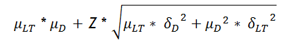
The key point is that the classic equation used to calculate inventory safety stock is flawed because it assumes a Normal distribution. See these links for confirmation that a Normal distribution is assumed and that the calculations are based upon the mean and standard deviations.
http://en.wikipedia.org/wiki/Safety_stock http://www.inventoryops.com/safety_stock.htm
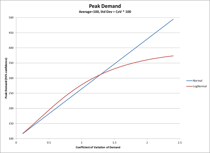
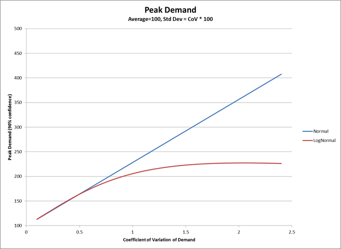
Each of these articles uses the mean and standard deviation of both demand and supply lead times, as well as the Z factor from Gaussian or Normal distributions. If we determine safety stock based upon the average demand, which is the usual manner of determining safety stock, we are keeping too much inventory to satisfy ‘most’ demand – as measured by the mode, or peak, of the distribution – and yet too much inventory to satisfy peak demand – as measured by the upper 95% confidence limit. As illustrated by the graph below, for a 95% confidence limit, once the CoV is above about 1.3 demand (that follows a LogNormal distribution), it would have a lower peak demand than demand that follows a Normal distribution. At a CoV of 2.5 the Normal distribution over-estimates the peak demand by nearly 36% using a 95% confidence limit, and by over 86% using a 90% confidence limit. Since safety stock is used to mitigate against the risk that we will run out of inventory to satisfy peak demand, clearly we are carrying too much stock in the cases where demand follows a LogNormal distribution. The same can be said for supply lead time where we are over-estimating the risk of not being able to get supply in time.
And it’s not just about demand and supply But it isn’t only demand or supply that follows a LogNormal distribution, or some other skewed distribution. In a paper titled “Log-normal Distributions across the Sciences: Keys and Clues” the authors point to many natural processes that follow a LogNormal distribution. In manufacturing we see skewed distributions for failure rates, yield, lead times, and many more variables. And yet we model all of these as single values in our planning systems and assume that if there is some variability that it follows a Normal distribution. The consequence is that we over-compensate with inventory and capacity buffers without truly understanding the associated risks. We would be far better off reducing these buffers and adopting a much more agile approach that accepts that occasionally shift happens. Plan for the expected and adjust to the exception. Side note: For those of you interested in running the experiment to determine how many negative samples will be drawn from a Normal distribution with different CoV, the code is below can be dropped into Excel provided you rename one of the worksheets “Norm_Inv”: Sub getCount() Dim i As Integer Dim j, n As Long Dim r As Single On Error Resume Next With Sheets("Norm_Inv") For i = 1 To 350 n = 0 For j = 1 To 1000000 r = WorksheetFunction.Norm_Inv(Rnd, 100, i) If r < 0 Then n = n + 1 Next j .Cells(i + 1, 2) = i .Cells(i + 1, 3) = n Next i End With End Sub More blogs in this series: Truth, Lies, and Statistical Modeling in Supply Chain – Part 2 Truth, Lies, and Statistical Modeling in Supply Chain – Part 3
Additional Resources
- Inventory optimization frequently asked questions
Discussions
Above all, this article--and, I would guess the series--will emphasize for all of us once again that supply chain agility, fast data, and collaboration will beat modeling and big inventories almost every time when it comes to producing what businesses are really after (i.e., making more money).
Making actual end-user demand visible across the entire supply chain and buffering with capacity rather than inventory in a supply chain that focuses on reducing replenishment lead times is movement toward eliminating entirely the vagaries and complexities of mathematical models. Most small to mid-sized business enterprises I know have no desire to hire a full-time statistician or mathematician to assure that they understand how their inventories are fully optimized.
I'm all for inherent simplicity. If managers and executives cannot explain in a couple of sentences precisely and accurately how their inventories and replenishments are calculated, chances are they don't trust the technology fully either.
Thanks again!
I have just one question.
You state: "If we determine safety stock based upon the average demand, which is the usual manner of determining safety stock, we are keeping too much inventory to satisfy ‘most’ demand – as measured by the mode, or peak, of the distribution – and yet too much inventory to satisfy peak demand – as measured by the upper 95% confidence limit."
Did you mean to say "...not ENOUGH inventory to satisfy peak demand...?"
Or perhaps I have misunderstood.
Thanks!
Yes, that is the exact point. Agility is the only way we can deal with demand variabiltiy and volatility, and this comes primarily from capacity buffers.
However, for companies with highly seasonal demand it is not feasible to build sufficient capacity to handle peak demand - unless they have an incredibly high gross margin - so there is still need to build inventory.
And from the capacity side the many of the same issues arise. While I love Eli Goldratt's The Goal, it is a simple fact that if yield and/or throughput are variable (and they are), not to mention capacity lost to setup, the capacity needed is roughly 120% of the throughput needed, depending on the yiled and throughput variability. Many factories and supply chains are built assuming a non-variable yield and throughput and therefore cannot achieve the desired throughput.
Regards
Trevor
Thanks, and sorry for the slow reply. I have been 'pondering' your question.
The answer is not as simple as I would like. The truth of the matter is that we are keeping too much inventory to handle confidence levels of peak demand - see the last 2 graphs - while at the same time we are under-estimating the risk of the getting unusually large demand. This is the point of the HBR article.
If the consequence of an unsually large demand is very great then it makes sense to either absorb the cost of carrying inventory for a long period of time that is unnecessarily high to deal with 'normal' demand. Or else establish systems and processes to detect the unusual demand as quickly as possible and absorb the cost in providing an agile and rapid response. Know Sooner; Act Faster.
Regards
Trevor
Where peak demands far outstrip capacities, techniques like dynamic buffer management (DBM) can still improve customer service levels while maintaining an inherently simple approach to inventory and production management.
This is especially true if MAX order size, MODE order size are taken into consideration in the course of establishing and maintaining buffer sizes and replenishment time is actively driven lower.
If peak demand is seasonal or cyclical, then the institution of build-up and build-down cycles based on peak demand quantities and capacity limitations also work well.
Thanks again for your great contributions at Kinaxis Community.
Truly,
Richard
It is probably also worth pointing out that much of the ill effects suffered by far too many supply chains could be eliminated through the adoption of policies that would remove the causes of many of the "peak demands"--versus more level demand. Many dramatic fluctuations in demand are self-induced and harmful.
For example, WalMart levels its demand and reduces supply chain troubles by offering "everyday low prices" rather than by offering large, short-term price reductions. Following that pattern, many supply chain participants could dramatically reduce supply chain problems--especially the negative affects of "the bullwhip"--by dropping policies that offer month-end, quarter-end, model-end or other short-term price reductions or incentives to the sales force. This approach to sales management tends to increase the occurrence of demand peaks, but lower prices, increased incentive pay-outs, and (sometimes) overtime or additional overhead incurred to produce, pack and ship in peak demand periods result in no great increase in profitability in the long-term.
Supply chain participants should work toward the elimination of self-induced supply chain headaches by establishing polices that do NOT introduce artificial peaks and valleys in demand. This would go a long way toward helping them stabilize their supply chains regardless of methods used to manage inventory and production.
What do you think, Trevor?
-- Richard
Yes, I agree, but ...
What has happened over many years is that the buffers - both inventory and capacity- have been reduced in the pursuit of better financial performance, while at the same time demand has become global and outsourcing/off-shoring has lengthened the supply lead time.
The other trend that is making this tough is the need for 'long-tail' products through differentiation. Other than for a few niche brands such as Apple, it is a long time since Western brands could design for the West and sell in the East. They have to design for both markets meaning product proliferation and therefore additional suply chain complexity.
So you are correct that we should always aim to remove self-induced volatility, but the nirvana of a level loaded factory driven by Henry Ford's dictate that "They can have any clor as long as it is black!" is long gone.
My 2c.
Regards
Trevor
The thing about using averages is that it's just that, an average. It can predict what is most likely to happen, but most likely isn't a guarantee. As people have mentioned in the comments above, that's why agility is so important. You can plan for the most likely but what do you do when the opposite occurs?
You are correct, but clearly I did not articulate the importance of first understanding that variability has a big impact on the efficiency of a system, and second understanding that the characteristics of the variability have a big impact on the manner in which one will address the impact of the variability.
That is the whole point of the LogNormal probablility density graph in which each line has an average of 100, but very different variances.
My take is that we can make huge improvements in agility by reducing the decision/information cycle radically and, in many cases, without impacting the physical supply chain much. It is all about getting the early warning to chnages that have important consequences and being able to evalaute the financial and operational impacts of decisions in a short time, well within the customer's expectation.
So you are correct, that we "can plan for the most likely but what do you do when the opposite occurs?"
Regards
Trevor
Having spent a great deal of my career in the retail world, I can relate very closely to Richard's hypothetical example of Walmart. Self-induced supply chain headaches, indeed. We can bullwhip ourselves into a quivering mass of blood and guts if we are not careful,
It has long been my belief that when we are working in a retail world that is dominated by "limited time offers" as opposed to EDLP (every day low pricing) that each and every promotion must be assessed on its own merits. By that, I mean that a collaborative forecast must be developed virtually at SKU level that incorporates variables such as absolute level of price reduction (e.g. $100 off), relative magnitude of price reduction (e.g. 25% off versus 50% off), length of promotion, positioning and size of ad space, media, product life cycle, underlying base demand, trend, and seasonality.
Companies run into real danger when managing a business that has been used to price stability for a very long time, then adopts off-price LTO marketing strategies. Their forecasting systems have typically not been designed to manage this kind of promotional activity, and the mind-set has not been ingrained into the forecasting culture. I have been there and lived the nightmare. The good news is that best forecasting practices can be brought into such environments.
Thanks again for the discussion!
John
I came across your blog post at random while looking something up on the internet. As a physicist turned operational researcher, I enjoyed your post, but I feel that it misses the mark a touch.
First, stochastic demand does not usually follow a lognormal distribution and in real operational research, no one assumes the normal distribution for demands or lead times in inventory control. The lognormal has lots of interesting properties, but stochastic demand tends to be better approximated by a compound Poisson process, an inhomogeneous Poisson process, or the negative binomial distribution. There is a deep set of motivating principles that suggest that these distributions capture demand processes well, but of course there are other distributions that practitioners use. It depends on the problem,
While we can model demand parametrically, in many inventory cases we do not need to do so. Non-parametric estimation methods applied to data can help us understand relationships that parametric methods miss (especially if the data is censored, which is a persistent problem with inventory) .
In the end, inventory control is an optimal control problem solved by dynamic programming and this is true whether the problem is deterministic or stochastic. The solution to the dynamic program gives you the optimal policy and it will tell you what your safety stock will look like. Demand estimation is just one piece of the puzzle - the hard part is solving the dynamic program as close to optimality as you can! (Unless you get lucky and simple (sS) polices work out of the box for the problem on hand - which is surprisingly often.)
Finally, I disagree with your statement that we usually use average demand to set reorder points or safety stock. The reorder point is set through the solution to the dynamic program and that depends on how stock-outs, holding costs, and back order costs are treated. In simple (sS) polices, the reorder points are set at quantiles of the underlying distribution (with no assumption about normality) that are functions of these inputs.
PS: As "highly" random as the lognormal might be - the stock market is even more random. The Black-Scholes equation for option pricing assumes assets follow the lognormal and the world is definitely not Black-Scholes!
In a great many organizations, the safety stock level is directly proportional to how much hell was raised by management last time the SKU suffered an out-of-stock (especially for a key customer or critical order) and inversely proportional to how much hell was raised by management over "too much inventory." Equally important in this equation is, which hell-raising occurred last--the "too much inventory" or the "out-of-stock" hell-raising.
I agree, this is a complex formula, but it has helped many an inventory manager or buyer keep his job while being tossed back and forth between the demands coming from sales and the demands coming from finance.
All contributions are greatly appreciated.
The point of my blog was that small amounts of variability - in demand, lead times, yields, etc - have a big impact on the performance of a system, and for the most part, we model our supply chains using single numbers - usually averages - and no indication of variability by scale and characteristics. This leads us to overestimate the peak performance of a system and to underestimate the risks.
I used inventory policy setting as an example of a mechanism used to cope with the variability. Could you share with the rest of the readership some more on how you go about planning inventory? Perhaps some links to articles?
Yes, I am aware that there are a plethora of different statistical functions that can be used to model demand. I probably should have been more explicit that my intent wasn't to suggest that the LogNormal is the only distribution to use, but rather that the behaviour it models is a lot closer to the real world than a Normal distribution. I was looking for a simple way to describe a complex problem, not to give a course in applied statistics.
Again, thank you for the lively discussion.
Regards,
Trevor
Love your comments because they bring out a key point about modeling of any system, whether a supply chain or not. This is that the model can never fully describe the behaviour of the system nor can it fully describe the decision making process of management.
In your example Richard, who is to say that management wasn't correct in both cases? At one time they may have needed the revenue when instead they suffered a stock out, and at another time they needed to reduce working capital so they could invest in product development or marketing. I wish that I could have absolute confidence that management were acting rationally every time they make a decision, but that is besides the point.
It is a complex issue to solve. The "any color as long as it is black" approach of manufacturing is no longer tenable. And yet I agree completely with both of you that we should reduce self-induced variability as much as possible. The same is true of product portfolio complexity. It is not a simple matter to determine how much complexity is required to meet market demand and differentiation while not introducing too much complexity and cost to the supply chain. In the 1990s one car manufacturer had 104 models and 98 different gas caps. This is needless product complexity.
I don't believe these issues can be 'optimized' with a purely mathematical approach. As I wrote earlier, the model is never complete and the decision process and variables can never be described fully. And, oh yes, there is that damned uncertainty in demand, and all the variables, for which we have not accounted fully.
It's not that these approaches tell us nothing and shouldn't be used. They are directionally correct. I get worried when people think they are absolutely correct because someone slapped the term 'optimization' into the description.
Regards,
Trevor
-- Richard
I agree with your assessment that the lognormal illustrates variability better than the normal and I liked your post's emphasis on the corrupting role variability plays in inventory control.
In my work, we provide insight into optimal policies for our clients. The idea is for us to learn something from the data. We go about our work by starting with simple models and seeing how much of the problem we capture. We continue to add complexity until we see no benefit. That is, we don't try to solve some complicated model to 0.5% of optimal when the inputs have 5% errors. But we do use fairly sophisticated Bayesian learning techniques to gives insight into the demand structure. We give our clients a deep understanding why a set of optimal policies for their inventory control looks they way it does.
As a reference for your readership, I suggest starting with Zipkin's book, Inventory Management.
The important point is, as Box pointed out so many years ago: All models are wrong, but some are useful.
Yes, I have used that quote from GEP Box several times. It is scary when people begin to believe that a model is 100% correct. Heck, even 90% is scary.
I really like your incremental approach based on insight and learning.
Thanks for the reference, and good hunting. http://www.amazon.ca/Foundations-Inventory-Management-Paul-Zipkin/dp/0256113793
Regards,
Trevor
Bob Ferrari over are Supply Chain Matters (http://www.theferrarigroup.com/supply-chain-matters/) pointed me to a webinar on Feb 6 by MIT's Center for Transportation and Logistics that brings up exactly the same issue - http://ctl.mit.edu/events/mit_ctl_ascm_ocean_transportation_reliability_myths_realities_impacts
In their case they are looking the port-to-port transit times for shipments from China to the US. One finding which interested me is that by comparison the dock-to-dock time is fairly consistent, but it was the in port times that were very variable.
This reminded me of a presentation by Imerys at a recent S&OP conference in Las Vegas on Jan 31-Feb 1 in which they discussed rail shipment times. The speaker said that they can string 25 railcars together in Georgia to ship the material to the same location in North Dakota and after 10 days 5 cars arrive, then anothe 5 arrive 3 days later, the 10 arrive a week after that, and when they make enquiries to the railroad they find that the other 5 are still in Georgia. On the other hand if all 25 had arrived at once it would have been a real problem for them because they would have had to pay $300/day in demurrage charges for each railcar.
Tough to manage this very effectively. My view is if they could know sooner and act faster to the real locations of the rail cars they could run their operations a lot more effectively.
-- Richard
Great blog. Incredible how the field has mature since the early days of Supply Chain Planning.
Control theory (and a supply chain system is just algorithms trying to "control" the supply chain) has recognised this for a while. The more uncertainty in the system the less performance we can expect and the simpler the controller should be.
Great to hear from you. It's been a long time.
What is amazing about your comment is that way back in the late-1980s, while working for Systems Modeling, who developed a discrete event simulation tool, I tried to apply Control Theory and Stochastic Optimization to manufacturing planning. It was just too slow and planning had no yet reached that level of sophistication. To be honest I knew far too little about discrete manufacturing at the time and tried to apply process concepts to a discrete world blindly.
I'm leaning more to Systems Theory and Complexity Theory to understand how a supply chain - really a network - behaves. And I'm not yet convinced that simple PID control systems can deal with the levels of uncertainty and nuance experienced in supply networks.
Regards
Trevor
Very interesting post and discussion, causing even a frequent lurker like myself to come to the surface!
As a supply chain practitioner and, more recently, a novice student of the social sciences, I have come to regard supply chains as "social structures" that exhibit "phenomena of organized complexity" (http://www.nobelprize.org/nobel_prizes/economics/laureates/1974/hayek-lecture.html).
As a result, supply chain management, like economics, sits uncomfortably between the physical and social sciences and has to deal with the problem of managing systems that are too complex to ever fully describe or comprehend.
Continuously questioning and perfecting the quantitative methods we use to understand and manage supply chains is no doubt part of the answer. However, this has to be complemented by a healthy dose of skepticism towards "overmathematising" and more focus on behaviors/methods/tools that allow fast access to information and responsive decision making.
"If man is not to do more harm than good in his efforts to improve the social order, he will have to learn that in this, as in all other fields where essential complexity of an organized kind prevails, he cannot acquire the full knowledge which would make mastery of the events possible. He will therefore have to use what knowledge he can achieve, not to shape the results as the craftsman shapes his handiwork, but rather to cultivate a growth by providing the appropriate environment, in the manner in which the gardener does this for his plants."
Every economic interaction is, first and foremost, a social interaction and merely an exchange of value. That is to say, the determination to exchange cash for goods and/or services is not predicated upon some independently determined or even independently verifiable scale of value. Rather, it the willingness to participate in an economic exchange is determined by dozens--perhaps hundreds--of calculations of value done independently by the participants. Each participant is comparing the value of participating in the exchange with the infinite range of possibilities for alternative uses of his or her time and money.
Therefore, efforts to optimize the level of supply chain collaboration must be built upon recognizing and communicating to participants (or potential participants) how they can optimize their own individual benefits ("marginal utility") while, at the same time, benefiting the entire supply chain (the "system"). This goes way beyond mathematics and requires actually getting to know your supply chain participants on a somewhat intimate level, in my opinion.
While Boolean algebra can help solve the puzzle of Game Theory, only intimacy can provide you with an understanding of the subtle variables involved in the actual game; and the game changes when the players change.
Good discussion where everyone is right.
Indeed every forecast is wrong, therefore we need the factor " human" and the system " communication" .
If these are able to work together than it migt be possible to get an agreement or even better a desiscion on the forecast and eventually the stock level. As long as these are well thought through and accepted by all stakeholders, both supplier and customer are satisfied. And if your lucky you can earn some money as well.
Great to hear from you after all these years. Don't lurk so much. You have a voice.
For so many years we have approached supply chain management from a reductionist perspective and thrown optimization at the problem on the assumption that the model is correct, when in fact, as per the quote from Hayek you included in your second post, we can never have full knowledge. And breaking up the problem only makes things worse.
But since we have taken such an "overmathematising" approach to SCM for the past years, I decided to approach the problem from a mathematical angle - statistical actually - to prove that some fundamental assumptions we use to calculate things like inventory are incorrect.
I did this because it is only once we have relinquished the quest for the holy grail of a 100% accurate mathematical model that we will begin to focus on the Human Judgment aspects. While we cling the idea that a computer can tell us the perfect answer we will not focus on the process and system capabilities required to enhance decision making through collaborative processes.
Plan + Monitor + Respond = Breakthrough Performance.
Planning is only the beginning. And no longer enough on its own.
Regards
Trevor
PS: there is also a lively discussion on http://www.linkedin.com/groupItem?view=&gid=56631&type=member&item=219437600&qid=58b1b5ee-0af4-4e82-9e5d-5a688113b56e&trk=group_most_recent_rich-0-b-ttl&goback=.gmr_56631
I could not agree more!
Thanks. I do get on the pulpit a bit. (get the reference?)
I think we need more than intuition. Please have a look at this blog I wrote on seredipity: https://blog.kinaxis.com/2012/11/serendipity-and-the-supply-chain/ Serendipity is 'trained intuition'.
Regards
Trevor
In our SS calculation, we're measuring Standard Deviation of Forecast Error, not of the demand itself.
Does your concern still apply?
As an example, you mention a typical absence of negative demand in the supply chain.
In our model, we frequently experience negative Forecast Error. Does this "re-legitimize" the Normal Distribution?
Thanks,
Ethan
In my opinion, measuring forecast error is like closing the barn door after the horses are out. How do you know what caused the forecast to be wrong? Finding out that one has a "fever"--and every forecast has a "fever"--only does one a service if you know the cure or how to discover the cure. Unfortunately, forecast errors are pervasive and measuring them tells you nothing about the cure.
Actually, truth be told, there is no "cure" for forecast errors. Purchasing requires a single-number forecast (not a range), and that number is ALWAYS wrong. (Or, if it is right, it is right only by chance, and is not repeatable as "right.")
The answers lie in other directions. Consider what is covered in the series that begins here, if you will: https://community.kinaxis.com/people/RDCushing/blog/2013/04/05/on-demand-driven-supply-chains-ddsc
I would not recommend using Forecast Error, one of the reasons being, as Richard mentions, that you do not know the cause of forecast error.
More importantly though, imagine if you had zero forecast error and a demand CoV of 5. Would this mean that you would carry 0 inventory? I doubt it very much because that would mean you would need infinite capacity. (See part 3 of my blog series.)
It just so happens that a high CoV usually results in high forecast error, but the opposite isn't true. Which is where Richard's point comes to play. Imagine you had 200% forecast error and a demand CoV of 0. Would this mean that you need large SS? The only inventory I would carry is cycle stock to balance replenishment and delivery lead times.
Hope this helps.
Regards
Trevor
I don't understand the relevance of calculating Demand CoV when I am using weekly Standard Deviation of Forecast Error in my SS calculation.
I do calculate CoV, but for a completely different metric.
Example: so what if I have ridiculously high CoV if the customer is frequently, or always purchasing exactly to that forecast? Believe it or not, this happens in my supply chain. This is the main reason I don't agree with the basis of Richard's post: that the "forecast is ALWAYS wrong".
Note that I am referring to internal nodes in the company. An assembly level node buying from a cost center node. This is very far upstream from any external customer behavior.
I'm suggesting that Std Dev of forecast error (FE) is not the correct way to go.
But assuming that you will stick with this approach, I would include a Forecast Bias metric too. It is very difficult to predict what shape FE will take. You really need to have a look at a histogram and a statistical test to determine if FE Normally distributed. If you are using MAPE and the CoV of FE is > 0.2 then you know it isn't normally distributed. :-)
There seem to be some words missing in your second paragraph. Can you retype it so I can understand your point?
I don't think it matters wehre you are doing the analysis, though there is less ability to change the behavior of an external customer in order to reduce demand variability.
Regards
Trevor
The node of the supply chain for which I am designing safety stock is as far upstream in our supply chain as one can go. It is an internal manufacturing center that produces low level components for next level assembly operations.
The point is that there is much happening in between "external customer" (customers buying our finished product 20 levels above me) forecasts and the demand signal we're looking at. We're not victims of customer forecast in the traditional sense; where one would characterize it "always wrong".
Your last sentence is very important. There is much I can do with the node above me to build a more predictable replenishment cycle; things one wouldn't normally try with an external customer; at least not in our business.
I plan to look at the distribution of Demand Error to see if it is normal. Remember, it will be distributed around the average Demand Error, not the average demand; which brings me full circle to why I originally posted. Measuring demand variation around the average demand is nearly worthless for the purpose of setting safety stock, but that seems to be the focus of your blog post; which is why I am struggling with it a bit.
I did not understand this part of your previous comment: "...ridiculously high CoV if the customer is frequently, or always purchasing exactly to that forecast?" It doesn't seem to be a complete sentence. Do you mean the customer is changing their forecast frequently?
I get the point that you are looking at the mean forecast error and standard deviation of forecast error. But if you have a MAPE that varies between 5% and 50% with a mean of 40% it is very unlikely that you have a MAPE that is Normally distributed, but you may if the 5% is an outlier.
The problem with MAPE is that is doen't tell you if you are over forecasting or under forecasting on a consistent basis. This is where Bias comes to play.
We have a different opinion about whether to use demand variation or forecast error. I think forecast erro is meaningless, and you think demand variability is meaningless. Can you explain why demand variation is worthless in your opinion? I tried to explain my point of view above:
"imagine if you had zero forecast error and a demand CoV of 5. Would this mean that you would carry 0 inventory? I doubt it very much because that would mean you would need infinite capacity. (See part 3 of my blog series.)
Imagine you had 200% forecast error and a demand CoV of 0. Would this mean that you need large SS? The only inventory I would carry is cycle stock to balance replenishment and delivery lead times."
Regards
Trevor
The complete sentence, as written above, is this:
"Example: so what if I have ridiculously high CoV if the customer is frequently, or always purchasing exactly to that forecast?"
I admit it is a poorly written sentence. But if one understands the use of the colloquialism "so what", then it shouldn't be too confusing.
My point is that if the forecast at lead time is extremely variable, I may not care as long as the node above me is buying to that forecast. I would need very little SS.
This is why Standard Deviation of Demand is not useful for calculating Safety Stock.
Variable Demand is no guarantee of stock out. A customer buying more than their lead time forecast (Forecast Error) is. The latter is what we want to protect against.
You're focusing on Forecast Error as a percentage. This is incorrect. Standard Deviation of Forecast Error Weekly is what we are interested in. This gives us an understanding of the distribution of error around a mean on a weekly basis.
If I had a demand signal with no variation, and the customer consistently bought more or less than their forecast, then I would carry SS. You say 200% error, but I don't know what that will look like on a distribution; so I don't know if I would carry "large" SS, or something more reasonable.
Demand variation is not worthless; as a separate metric. I have a Demand Variation & Trend metric (http://supplychainmi.blogspot.com/2012/02/taming-bull.html). I am only maintaining that it is near useless for calculating SS.
You are making the assumption that the demand lead time is greater than or equal to the supply lead time. In my experience this is very seldom the case, and that the supply lead time is constant.
Almost inevitably there are long lead times raw materials that have to be bought beyond order lead time, and frquently the manufacturing lead time exceeds the order lead time. For example, it is not unusual for the Pharma industry to have 6-18 month maufacturing lead times, and 2-4 week demand lead times.
My experience in High-Tech is that as demand goes up the supply lead time also goes up, maybe not in a 1:1 ratio and often with some lag, but there is a definite correlation. This si becuase companies - whether internal capacity or suppliers - do not have infinite capacity so as demand goes up so does lead time. So I have some questions when you write 'forecast at lead time'.
We may need to agree to disagree on Forecast Error vs Demand Variability. In your example, it is just as likely that another customer ordered an equivalent amount less so the net effect is no change in demand.
Regards
Trevor
I’m a real estate developer and noticed some distribution center & supply chain warehouse contractors/developers are employing statistical modelers now??? I’m not smart enough to understand why but they are the most successful developers I know. Can you offer any insight as to what they are looking at or how I can gather the same data??
My response here is a completely operational, and not statistical solution.
I implemented a global solution to address the challenge John stated. We took a different approach and it was very successful. Just to give a perspective, my company is a Network Equipment Provider, a global player. Suppliers are around the world. Contract Manufactures in China, Mexico, Chez, and the US primarily.
Given global consolidated demand, accuracy drops to 42% and segmented demand accuracy rarely reaches 70% in the best-case scenario, even with customer co-planning. The company had implemented Lean operations, and VMI already.
My approach was completely opposite to general practice, which is perfecting the demand forecast and then going after the supply commits. I based my solution on Harvard's article from the 1990s. Perfect the demand for the existing supply plan. Then go after perfecting the additional demand forecast. We worked on demand segmentation rigorously. For each segment, the identified variability needed in the statistical model.
Although the company has enough money power to hire statisticians, still a segmented approach and applying more than one operational solution paid off.
We worked with the suppliers and CMs on various fronts simultaneously. For example, Faster supply commit response, gross demand as consumed by each supplier. Short, medium and long term supply capacity visibility.
Leave a Reply