The RapidResponse platform is underpinned by a purpose-driven database engine that we developed at Kinaxis. On the Database Engine team, we maintain and continually improve the database engine. We frequently solve problems related to performance, parallelism, and memory management.
This blog talks about one of the first problems that I tackled when I started working at Kinaxis on the Database Engine team. The task was simple: Speed up one of our index builders. Let's take a look at some of the practical techniques we used to improve the performance.
Problem details
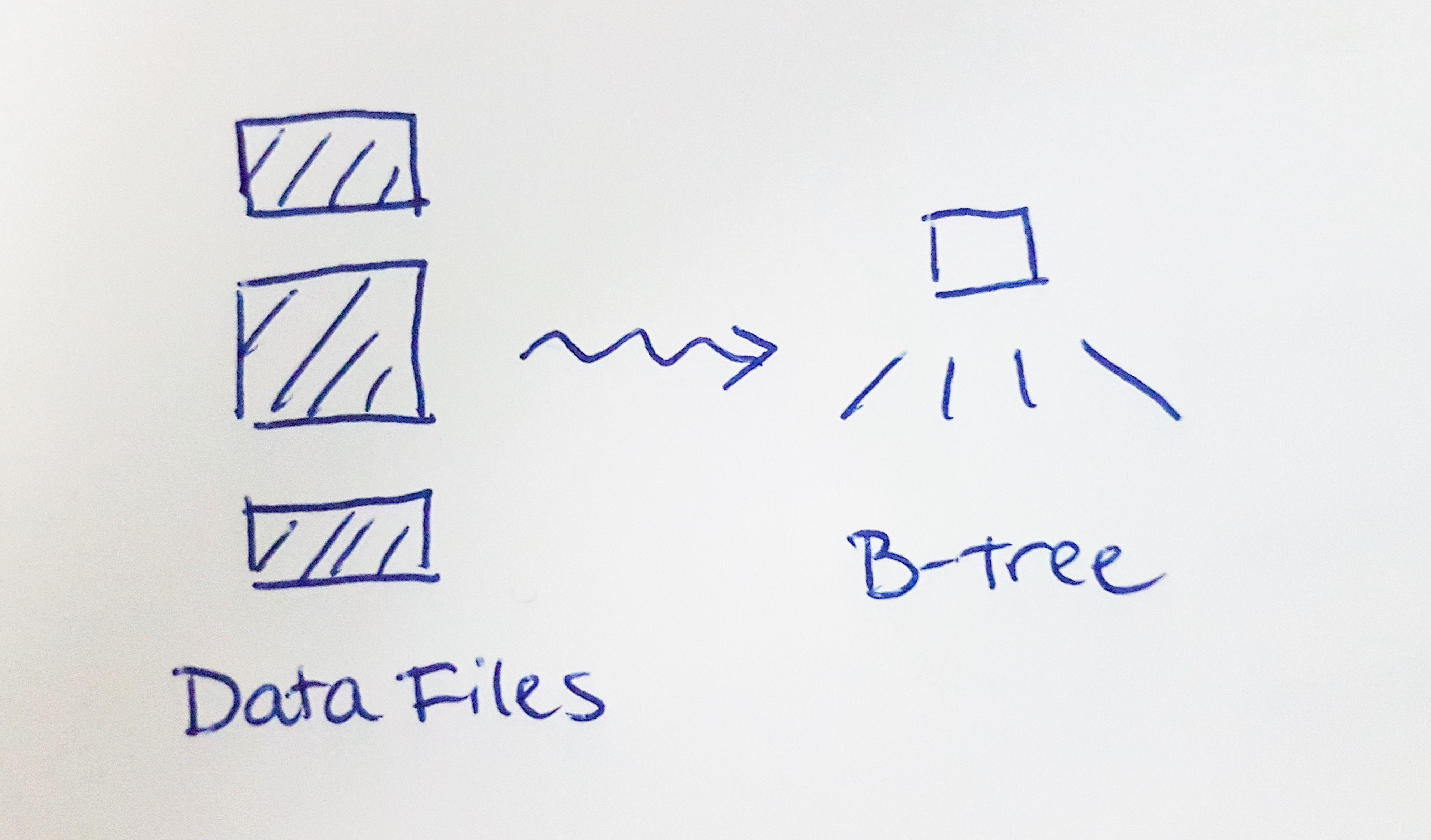
An index is a data structure that speeds up the performance of certain data access operations.
An index builder is a code component that is responsible for building an in-memory index from the on-disk representation of the database.
Here are some more details about this particular index builder:
• The in-memory index is implemented as a B-tree.
• The index must perform well for insertion and search.
• Index entries are basically 64-bit integers.
• The index builder scans a bunch of data files, extracts the index entries, and builds the B-tree.
• The data files being scanned are unevenly sized, each containing a random number of index entries.
• The index entries in the data files are unsorted, and include duplicate entries.
• There is a wide variation in the expected index size. A typical index index could contain 1, a few, or thousands of entries. The upper bound is around 10 million entries.
Original implementation
The original implementation of the index builder looks like this:
1) A single thread scans all the data files, extracts the index entries, and inserts the entries one-by-one into the B-tree.
A couple things in this implementation stand out as being expensive:
1) File scanning is slow.
2) Inserting entries one-by-one into the B-tree is slow, and difficult to parallelize.
Improvement 1: Parallelize the file scan
The first improvement is to parallelize the file scan.
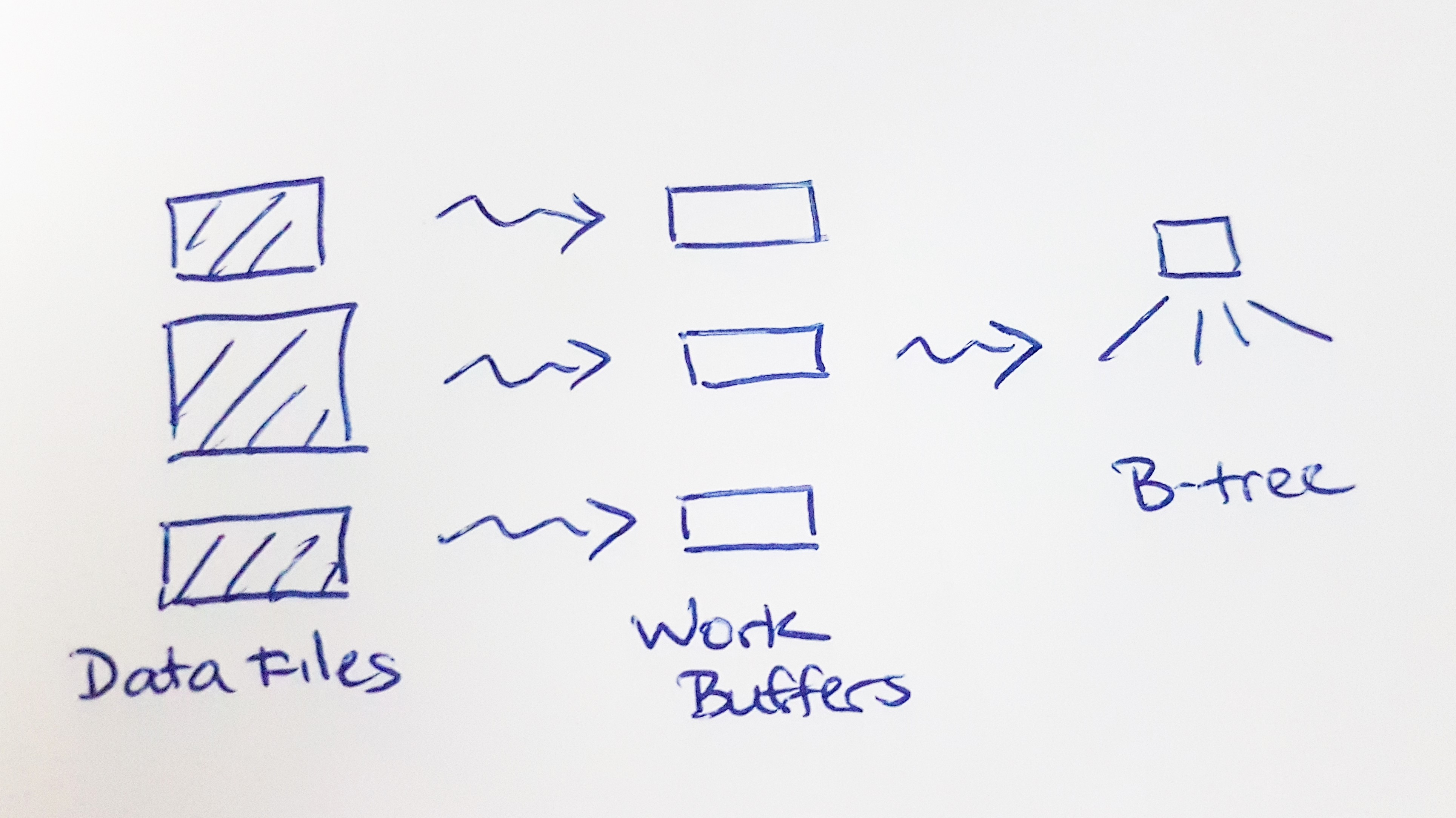
1) Divide the file scanning among a pool of worker threads.
2) Each worker thread extracts the index entries from its assigned set of data files and pushes them into a private work buffer.
3) Take the index entries from the work buffers and insert them one-by-one into the B-tree.
Parallel file scanning better utilizes the file storage device's throughput capacity and reduces the file scanning time significantly. We can also enable some parallelism between file scanning and inserting into the B-tree. However, performance is still majorly constrained by inserting into the B-tree, which must be serialized.
Improvement 2: Build the B-tree bottom-up
What makes B-tree insertion slow? An insert operation has to: traverse the tree, dynamically allocate memory for tree nodes, and rebalance the tree. Can we find a faster way to build the B-tree?
First, let's observe that we can build and sort an array-like data structure much faster than we can build a balanced B-tree using insertions. For example, let's compare these operations using the C++ standard library as a reference.
• The array-based approach uses std::vector, std::sort, and std::unique.
• The tree-based approach uses std::set.
Sample code: sort_vs_tree.cpp

constexpr size_t MAX_ELEMENTS = 10000000;

std::vector<uint64_t> dataArray;
std::set<uint64_t> sortedSet;
std::vector<uint64_t> sortedArray;

void GenerateDataArray()
{
     dataArray.reserve(MAX_ELEMENTS);
     for (size_t i = 0; i < MAX_ELEMENTS; ++i) {
          dataArray.emplace_back(std::rand());
     }
}
void BuildSortedSet()
{
     for (auto e : dataArray) {
          sortedSet.emplace(e);
     }
}

void BuildSortedArray()
{
     for (auto e : dataArray) {
          sortedArray.emplace_back(e);
     }

     std::sort(sortedArray.begin(), sortedArray.end());

     auto last = std::unique(sortedArray.begin(), sortedArray.end());
     sortedArray.erase(last, sortedArray.end());
}

int
main(int argc, char* argv[])
{
     std::cout << std::setprecision(3);

     Timer timer;

    {
         TimerContext tc(timer);
         GenerateDataArray();
    }
    std::cout << "GenerateDataArray " << timer.DeltaS() << "s" << std::endl;
    {
         TimerContext tc(timer);
         BuildSortedArray();
    }
    std::cout << "BuildSortedArray " << timer.DeltaS() << "s" << std::endl;
    {
         TimerContext tc(timer);
         BuildSortedSet();
    }
    std::cout << "BuildSortedSet " << timer.DeltaS() << "s" << std::endl;
    return 0;
}
For 10 million elements, here are the results on my development machine. The array-based approach is over 3.7x faster than the tree-based approach.
BuildSortedArray 3.99s
BuildSortedSet 14.7s
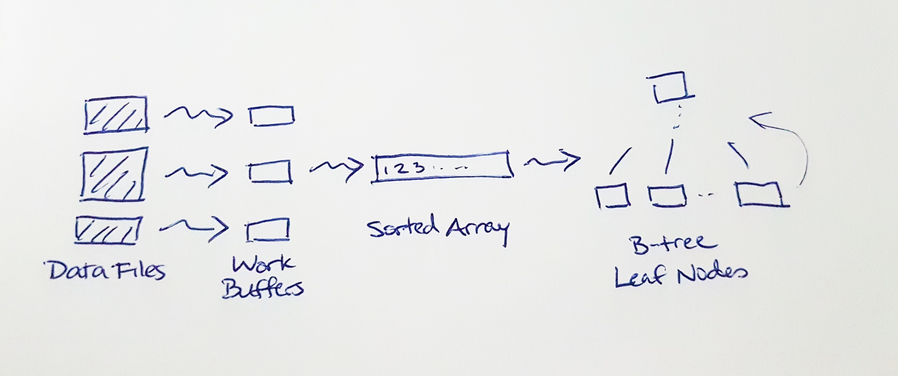
Once we have a sorted array of index entries, it doesn't make sense to insert them into the B-tree one-by-one. Instead, let's build the B-tree from the bottom, up. We start by dividing the sorted entries into leaf nodes, and then construct the tree structure above them.
Since we can calculate the height and number of tree nodes up-front, we can efficiently batch-allocate the tree nodes with the minimum number of memory allocations. We only have to assign each parent-child node link once. We never have to rebalance the tree, or split or combine nodes.
Now the index builder implementation looks like this:
1) Divide the file scanning among a pool of worker threads.
2) Each worker thread extracts the index entries from its assigned set of data files and pushes them into a private work buffer.
3) Merge and sort the work buffers into a single sorted array.
4) Build the B-tree bottom-up.
Next, we'll take a closer look at how the index builder manages memory.
Improvement 3: Optimize the work buffer data structure
Let's think about the implementation of this step, "Merge and sort the work buffers into a single sorted array." What data structure(s) should we use to implement the work buffers and the sort buffer(s)?
Since these data structures are arrays, we could naively choose to use std::vector. Some of the drawbacks of this approach are:
• A std::vector requires a contiguous memory allocation. This might be practical for a smaller work buffer, but not for a much larger sort buffer. e.g. An index of 10 million entries needs approximately 80 MB.
• If we need to grow or shrink a std::vector, we need to copy all of its contents from one contiguous chunk to another.
• The only way to merge one std::vector into another is to copy all of its data.
• std::vector allocates extra memory to mitigate the cost of growing, which can waste a lot of memory.
We decided to use a hybrid data structure, which is a linked list of small arrays. Here is the data structure definition.
template<int block_sz=30>
struct BufferNode {
        uint64_t mData[block_sz];
        uint64_t mUsed;
        struct BufferNode* mNext;
};

template<int block_sz=30>
struct Buffer {
        size_t mUsed;
        size_t mReserved;
        BufferNode<block_sz>* mHead;
        BufferNode<block_sz>* mTail;
};
The benefits of the Buffer structure are:
• We don't need to be able to allocate large blocks of contiguous memory.
• It is cheap to grow, and cheap to truncate.
• It is cheap to merge buffers. We just splice the BufferNode lists.
• We can bound the memory wasted.
It turns out that the Buffer structure is an effective way to implement both the work buffers and the sort buffers, because it complements the sort implementation we will discuss next.
Improvement 4: Adaptive merge sort
We need to choose an algorithm to merge and sort the work buffers. Given the nature of the problem, merge sort is an obvious choice.
Merge sort also works well with data stored in the Buffer structure because it accesses the data linearly. Quick sort and insertion sort do not work well because they require random access.
Recall that the expected index size is bi-modal: Some indexes may be small enough that std::qsort is perfectly adequate for handling them.
Since the unsorted index entries are likely to have small local runs, we can reduce the number of comparisons needed by organizing the merges by run. We can also produce runs by starting with std::qsort on fragments of the work buffers.
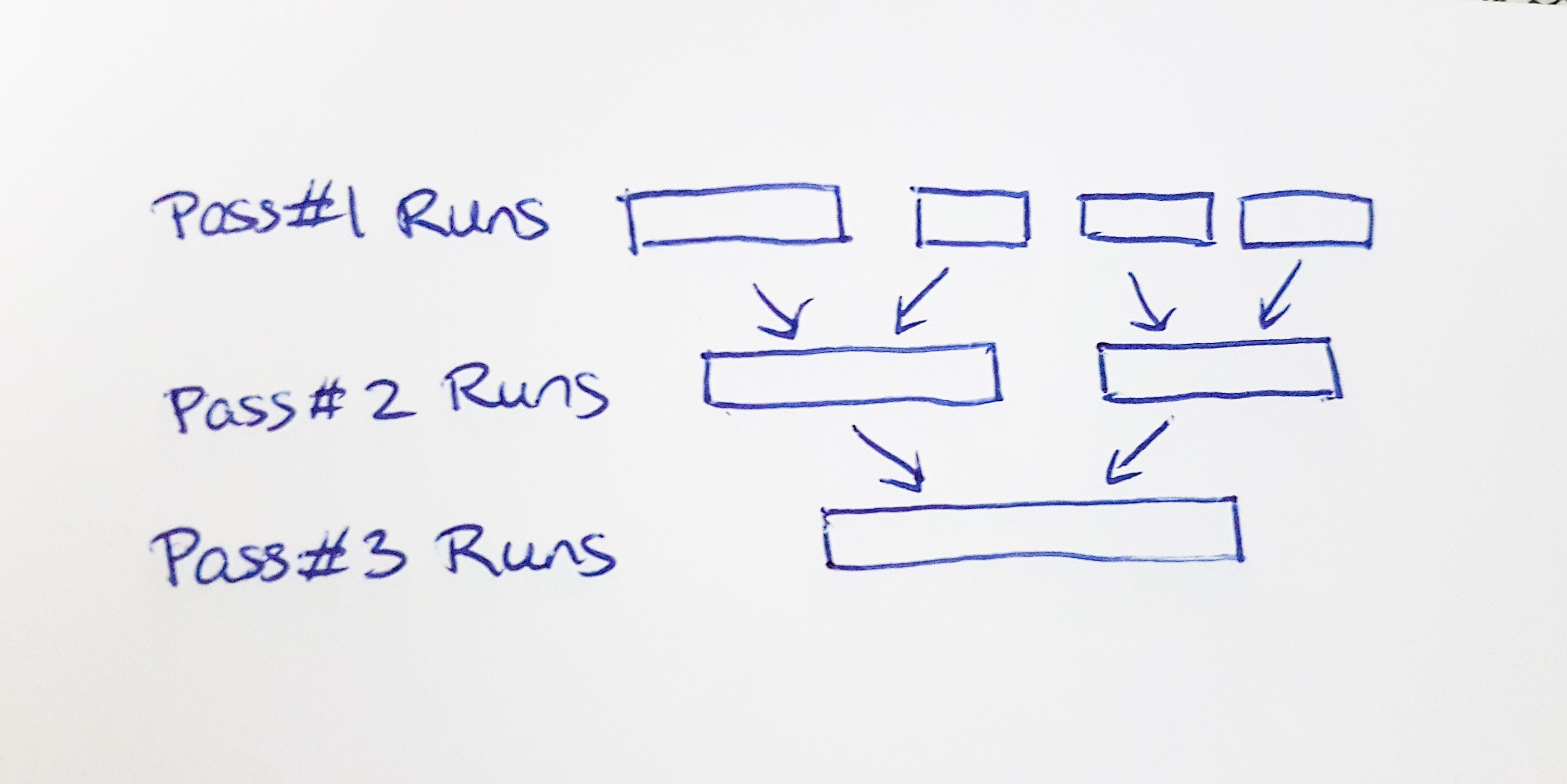
This leaves us with a simple adaptive merge sort algorithm like this:
• Sort and uniquify each BufferNode using standard library functions like std::qsort, which work well for small arrays.
• Splice the work buffers and split the initial unsorted index entries into runs.
• Walk through the spliced data in pairs of runs. Merge-sort each pair of runs into a longer run.
• Repeat step 3 until the data consists of only a single run.
Improvement 5: Optimize the sort memory management
Profiling showed that the only significantly expensive operation remaining in the sort phase was memory allocation. We can make a few last refinements to minimize the number of calls to the memory allocator.
1) Because the per-thread work buffers use the same Buffer structure as the sort buffers, we can easily splice the work buffers and reuse them as sort buffers. We only need to allocate one additional sort buffer.
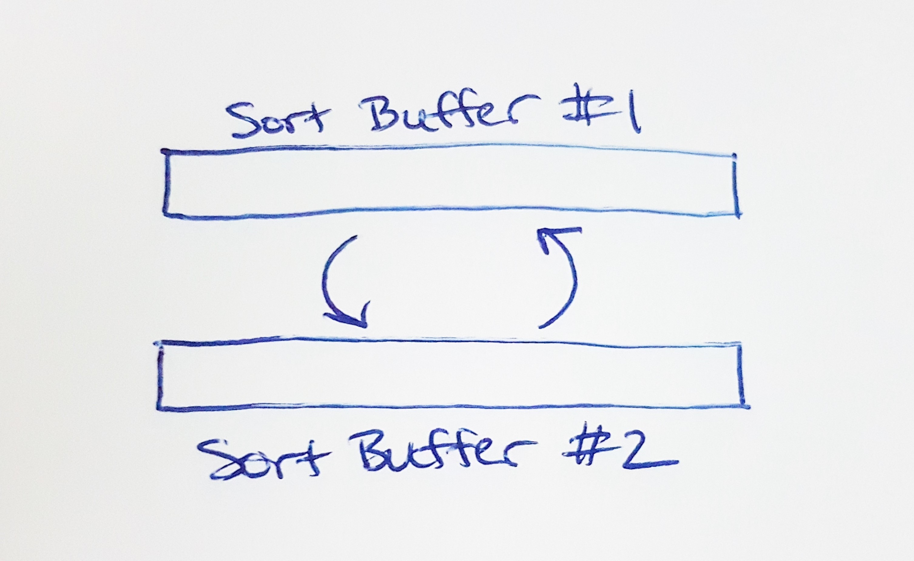
2) Each pass of the merge sort requires a source and destination buffer. Use a "double buffer" approach to reuse the same sort buffers for every pass of the merge sort. i.e. If pass N merges from buffer #1 into buffer #2, then pass (N+1) merges in the opposite direction, from buffer #2 to buffer #1.
3) Since we know the max possible size of the merged index entries, we allocate the whole sort buffer up-front. We also allocate large blocks of BufferNodes contiguously, which reduces the number of memory allocations needed.
Lessons learned
These are some things that I learned from this task.
• Manage your memory allocations. Memory allocation is expensive enough to dominate the performance of almost any straightforward algorithmic code. It is also likely to be a parallelism chokepoint. So allocate memory as carefully as possible.
• If an algorithm can be easily converted into a divide-and-conquer mode, then parallelizing it is the easiest optimization.
Finally: The choice to implement a custom sort algorithm is controversial. The overwhelming majority of the time, I recommend reusing an existing implementation. When I was working on this task, I was focused on the memory management, and the sort algorithm followed naturally from the data structure choices. I later learned that I did, in fact, reinvent the wheel – I had stumbled upon a primitive version of Timsort!
One last thing. If you like what you've read here and think we're the kind of team you'd love to join, Kinaxis is hiring! We'd love to hear from you. Visit: https://www.kinaxis.com/en/careers for open positions.