The importance of time series data for forecasting has long been a key area of research for academics and practitioners alike. Financial analysts rely on forecasts for understanding the ebb and flow of markets. Policy makers rely on forecasts to make decisions about production, purchases, and allocation of resources. Retailers rely on supply and demand forecasts for planning and budgeting.
In all these cases, inaccurate predictions can lead to economic downfall, losses for both consumers and producers, social distress, or poor monetary policies.
Statisticians led the work on forecasting for a long time. Regression and autoregressive (AR) models conquered for as long as data was hard to find.
These models, however, presented a naive view of time series – assuming they're linear when in reality, they’re not. Today, both data and computing power have become readily available, shifting the focus of both academics and practitioners towards machine learning (ML) models for forecasting.
While some have found significant success with classical ML solutions, others argue the need for deeper models, found in the study of deep learning (DL). Arguments backing ML rely on the relative simplicity of the models, compared to those found in DL. They also require less computing power, and hyperparameter tuning is generally simpler. Deep models, on the other hand, are great at modeling complex, non-linear, and hidden relationships in data.
In this two-part series on deep learning for time series forecasting, we'll aim to answer the following question: Are deep models needed for time series forecasting?
While the answer to this question can depend on your business's objectives, resources and expertise, the goal is to understand: one, just how big of a step it is to go from naive statistical approaches to more powerful deep learning models; and two, if it's worth it.
In this first part, we’ll analyze the performance of statistical models. Part two will cover machine and deep learning models.
Note: The entire notebook, with all the code, can be found in this public repository.
Analysis setup
Computing environment
All models will be trained and tested on a machine with 128 GB of memory and 32 cores, in a Databricks environment.
Dataset
We'll be using the bike sharing demand dataset from Kaggle, which can be found here.
It spans two years, is sampled every hour, and is set up such that the first twenty days of each month are used as the training set, while the last ten are used for testing.
Our forecasting goal will be to predict the number of bikes rented at every hour i.e., the count column. We can start by getting a high-level understanding of our data.
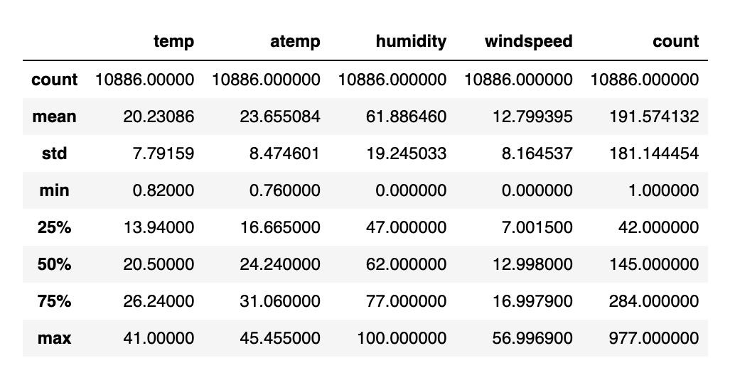
Table one gives us an idea of the data’s dispersion. The minimum value of zero for both humidity and windspeed is odd. It's likely that the values were very low, and as such rounded to zero.
We can deal with this by either predicting the windspeed using some machine learning model, or simply leaving it as-is. For the purpose of this blog, we'll keep the zeroes and assume that these values were initially extremely low.
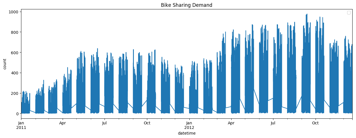
The line plot in figure 1 shows that there's clearly some yearly seasonality in our data, with lower demand during the winter season (January through April) and higher demand in the summer.
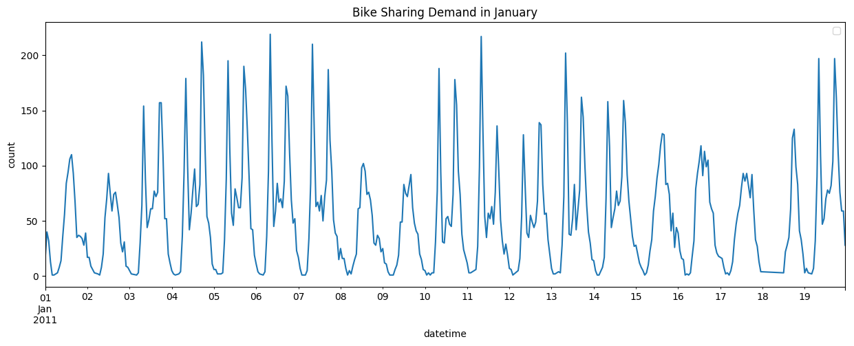
We can also zoom in on one month in particular, to see if there's any seasonality on a daily or weekly level, as is done in figure 2. Again, we see some seasonality at the daily level, likely due to the difference in demand on a weekday as opposed to on a weekend. As for trends, we don't see any. This information will become important later during our analysis of different models, as some models are better suited to work with seasonalities and trends, than others.
Finally, we split our data to have 90% of it in the training set, and 10% in the testing set, leaving us with approximately 9,800 training points, and 1,000 testing points.
Forecasting
We'll start our analysis by looking at some of the oldest models available for time series forecasting:
1. ARIMA: Model for univariate data that produces forecasts based solely on previous observations. External factors, such as weather, or the day of the week, aren't considered, nor are seasonalities. ARIMA takes as input three variables: Lag order, or p, degree of differencing, or d, and the order of the moving average, or q. What these variables mean is out of the scope of this article, but it's important to understand that they exist, and that they have significant impact on the results received.
2. SARIMA: SARIMA extends ARIMA. While it is still only suited for univariate data, this model includes extra terms that deal with seasonality. In addition to the three variables needed for ARIMA, SARIMA takes as input four more: seasonal P, seasonal D, seasonal Q, and the number of observations per seasonal cycle, m. Once again, what these variables mean is out of the scope of this article.
3. SARIMAX: Also an extension of ARIMA, but this model works with multivariate datasets. As such, it factors into the predictions the impact of external features on our forecasts. Along with the six variables used by SARIMA, SARIMAX also expects an array of features.
Selecting the right parameters for these models requires significant statistical background, and a good understanding of autocorrelation, seasonality, trends and ACF plots.
Luckily for us, there are libraries that can select the optimal values, based on our data. We'll be using the auto_arima function from the pmdarima python library to run these models against our dataset. The error metric we'll use to compare the different models will be the root mean squared logarithmic error (RMSLE). This is the metric used to judge the submissions to the Kaggle competition, where the leading results stand at an RMSLE of 0.33.
Let's see how the different models perform.
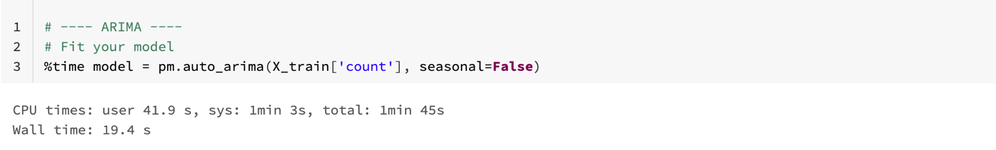
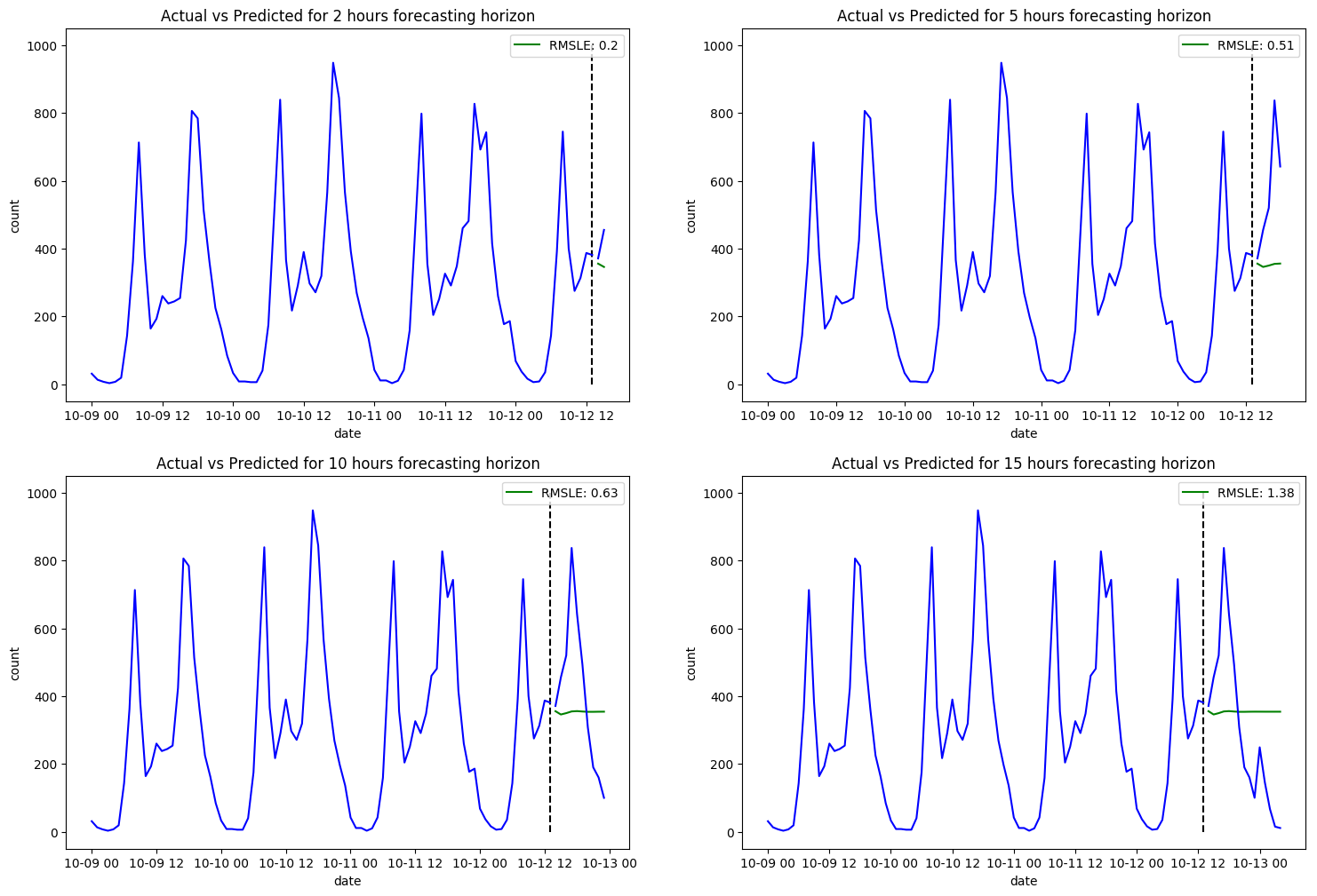
Figure 3 shows that ARIMA doesn't perform too well on our dataset, especially as we increase the forecasting horizon. In fact, it would have been naive of us to think it would perform any better than it has. Seasonality is a big factor when forecasting, but ARIMA doesn't include any seasonality terms, hence the poor performance. It also excludes any exterior factors that may be impacting the demand on bikes.
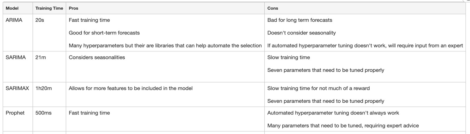
It's important to note, however, that the RMSLE for a forecasting horizon of two hours is relatively low. This indicates that for short-term forecasts, ARIMA can be useful, especially if we take more time to tune hyperparameters and clean our dataset.
The obvious next step is to include seasonality terms in our model, so let's see how SARIMA performs.
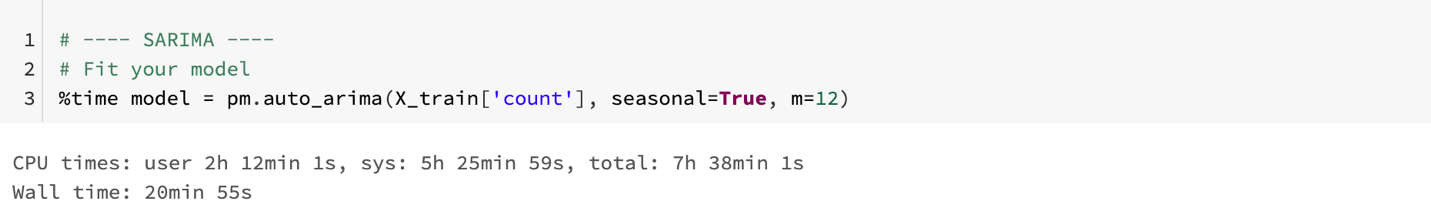
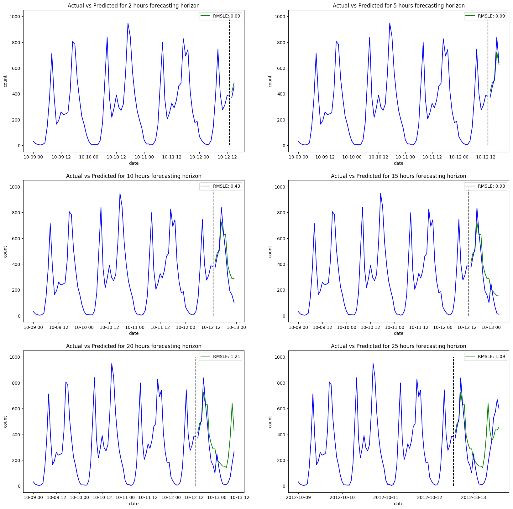
Definitely an improvement once we consider the seasonality in our data. Notice however, the much longer training time compared to ARIMA. Whereas it took only 20 seconds to fit our ARIMA model, the new seasonality terms have increased our training time significantly, to a total of twenty minutes. Considering our dataset is relatively small, this can become an issue if your goal is to scale. In terms of forecasting, this model seems to deal better with longer forecasting horizons, but still not convincing. The RMSLE gets higher as we pass the five-hour mark.
You'll notice also that we had to pass the number of observations per seasonal cycle (m) to the auto_arima function, since it isn't a parameter it can learn on its own. This adds an extra layer of complexity to the model, since setting the right m will need a good understanding of line plots, and how to spot seasonal cycles.
The final step, before moving on to a different class of algorithms, is to see how well we can forecast if we add extra features to our SARIMA model. As aforementioned, The SARIMAX model takes an extra parameter X, which is an array of all the features you want to feed your model.
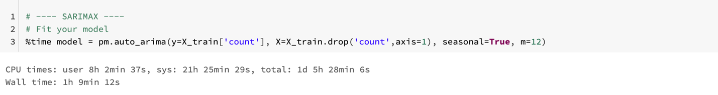
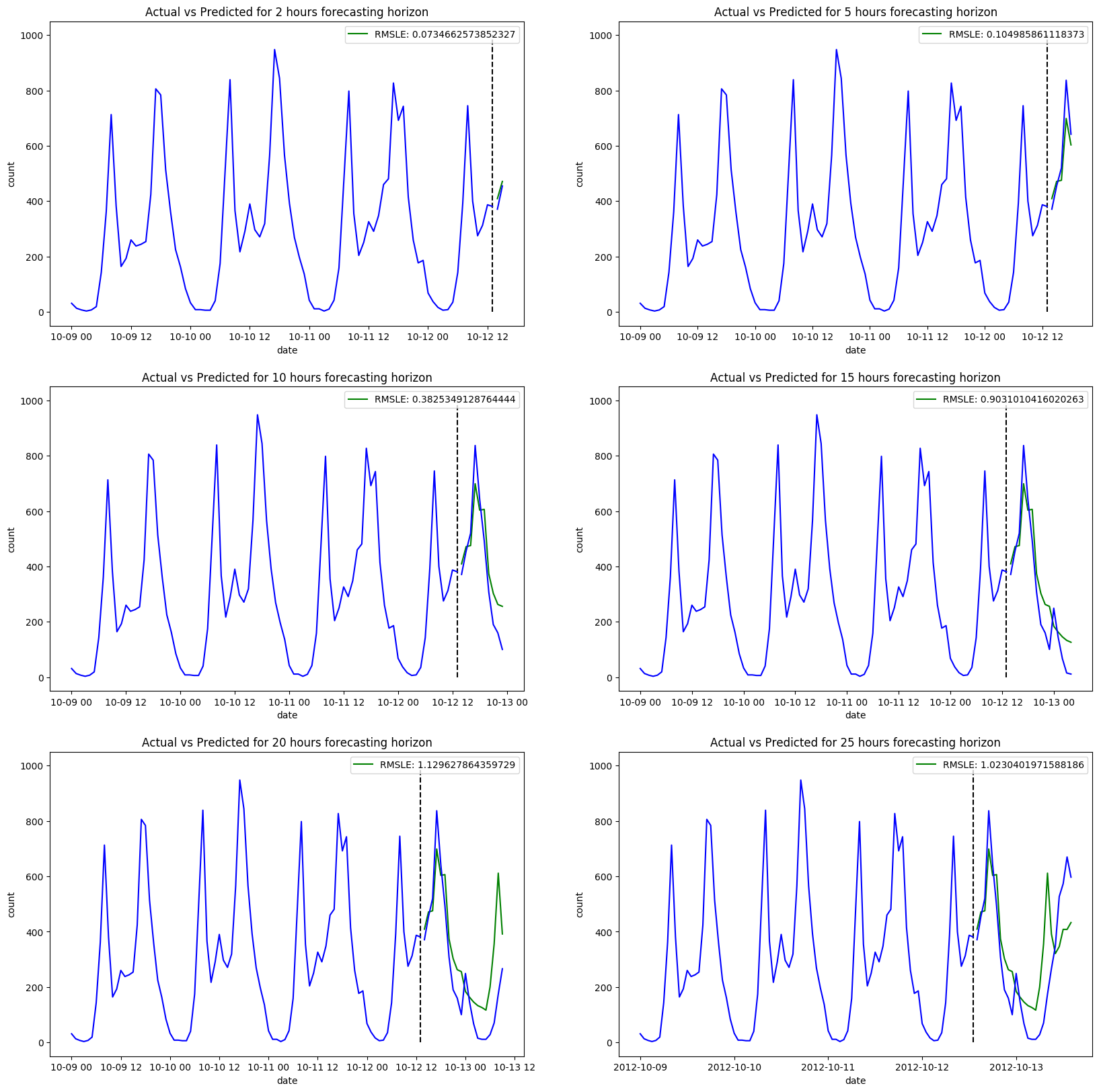
Immediately we notice a huge blow in performance, with the addition of new features increasing our training time to a whole hour and thirty minutes. Again, considering how small our training set is – compared to how large they normally are for large organizations – this increase in time is concerning. Even more concerning is the little reward we get back. Although we do see better results for both short- and long-term forecasting horizons, these improvements aren't significant.
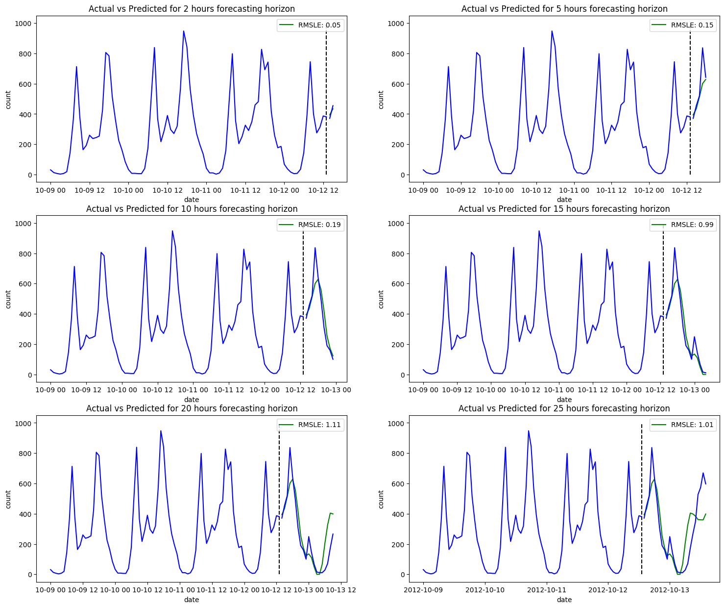
The next model we'll look at is Prophet. Prophet is Facebook's time series forecasting solution and is advertised as a model that is suitable for people who wish to produce forecasts but aren't experts. Facebook also claims that their solution is designed to handle a wide variety of forecasting problems. We'll put these claims to the test by using Prophet on our own dataset.
Before doing so, let's have a quick look at how the model is built:
y(t) = g(t) + s(t) + h(t) + E
Where g(t) is the trend function which models non-periodic changes in the value of the time series, s(t) represents periodic changes (e.g., weekly, and yearly seasonality), and h(t) represents the effects of holidays which occur on potentially irregular schedules over one or more days [1]. The paper on Prophet also mentions a Z(t), which is an optional matrix of other features we wish to add to our model.
A few points to make:
- After playing around with the different features that should be included, it was concluded that the features season, weather, working day and holiday greatly decreased the accuracy of our model, so we omitted them.
- The training time is extremely fast.
- A lot of hyperparameter tuning was involved. Like the ARIMA models, Prophet allows you to set most of the hyperparameters to auto, where the library will take care of finding the optimal hyperparameters. That being said, the seasonalities in our data weren't getting recognized, so we were forced to set them ourselves. The same goes for the number of changepoints, where Prophet was adding way too many.
- Finally, and most importantly, it seems like Prophet doesn't perform much better than SARIMAX did. Just like SARIMAX, it seems to struggle once it gets past the ten-hour forecasting horizon mark.
Conclusion
In this first part, we analyzed the performance of autoregressive models on the forecasting problem. While they were good for short term forecasting, they struggled as we increased the forecasting horizon.
More complicated models in SARIMA and SARIMAX came at the cost of a higher training time, with little benefit to the forecasting accuracy. They also involve more parameters, which implies the need for better statistical knowledge.
Prophet's training time was significantly better than that of SARIMAX, with similar forecasting results, so it can be used as an alternative to SARIMAX. This doesn't mean, however, that the likes of ARIMA, SARIMA and SARIMAX should be completely ignored. For smaller datasets, that aren't too complex, these autoregressive models can be very useful.
I leave you with the table below, which summarizes the results we got in this article.