Authors:
Stefan de kok, CEO of Wahupa and Masoud Chitsaz, Technical Thought Leader at Kinaxis
Uncertainty exists! What matters the most is how we make decisions.
Many businesses use advanced probability theory in action and these days it has become an indispensable part of their operations. Examples can be found in the applications of forecasting, risk management, and decision analysis. No surprise, there is no simple solution to these business challenges.
However, we can improve the quality of our business decisions by embracing uncertainty and applying the science of probability in the decision-making process. The intent of applying probability concepts in business operations is to get better knowledge about whether and to what extent events, actions, and outcomes are correlated. These concepts play a key role to determine the risk level of business actions in the face of uncertainties which helps decision-making to be data-driven.
The frameworks for making decisions under uncertainty can be of statistical or probabilistic type. Each of these frameworks can return deterministic or stochastic solutions that include confidence ranges for the decisions. Each type of framework and resulting solution has its use cases and benefits. Depending on the type of business decision, its criticality, and the availability of data, we can choose the proper type of framework and resulting solution category to employ.
A deeper understanding of each category and possible combinations will help to choose the right one for the business.
Deterministic vs. stochastic results
Some models produce deterministic results. These are exact numbers, and when used in planning are approximations of uncertain amounts. Often, they are some historical averages plus buffers to capture the variability and uncertainty. When applying such models with deterministic outputs repeatedly, we will get the same exact values for a particular set of inputs. The mathematical properties are known in this case. None of them are random, and each problem has only one set of specified values as  well as a single response or solution.
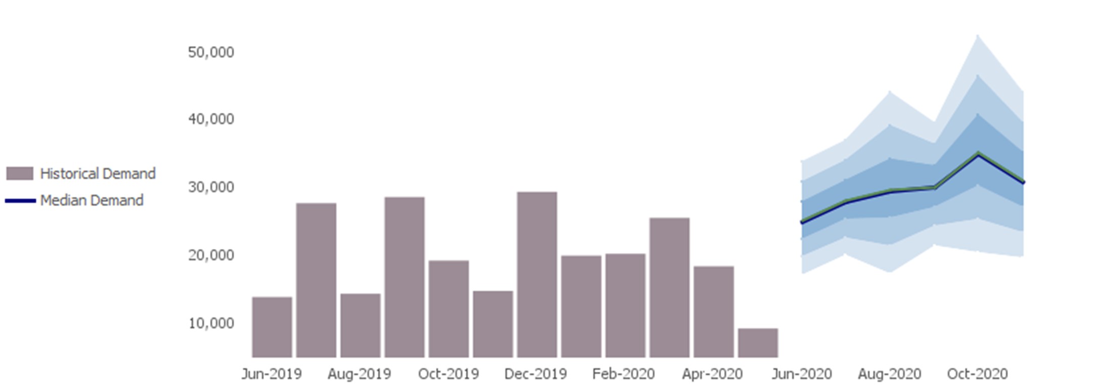
Stochastic results, on the other hand, depend on the probability distributions instead of exact numbers for any value representing anything uncertain in the future (Figure 1).
This could include quantities, lead times, production rates, yields, and so forth. Stochastic output is not guaranteed to be identical if the same calculation is executed multiple times, but only up to a given precision.
Statistical vs. probabilistic calculations
Obtaining the knowledge about the pattern of change and variation in various involved parameters is the first step when uncertainty is involved in controlling a system or making decisions for business operations. To do so, we can either use statistical calculations and use standard or well-known distributions or we can employ probabilistic methods and make little to no assumptions about the pattern of the distribution.
In the first case, we need to make strict a priori assumptions about the pattern of the underlying data. The two most common assumptions are that the data is exact or that it is normally (Gaussian) distributed. An example of exactness is a demand forecast expressed in simple numbers: next month we will sell 100 units of product A. An example of assuming a normal distribution can be found in all commonly used safety stock formulas, where it is implicit in both the service factor and the use of standard deviations on both demand and lead time. Both these cases, allow simple calculations, which explains their popularity.
The second case, probabilistic methods, comes in two main variants: parametric and non-parametric. Both have upsides and downsides. Parametric probabilistic methods are highly scalable and need little more data than statistical methods. They differ from the latter, mainly in that the parametric distribution first needs to be determined. And depending on which distribution is determined, parameters may be much harder to estimate accurately. An extreme example is to apply a Tweedie distribution, which can mimic almost any actual distribution, but is near impossible to fit accurately.
Estimating a distribution nonparametrically requires a large amount of data, especially continuous distributions. The question is how many data points do we need to properly describe an empirical distribution? Well, it really depends on the importance of the business problem and the level of precision needed in modeling the system. To get a better understanding, let’s look at a numerical example within the following chart.
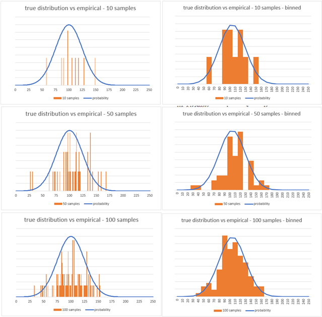
If we generate random samples for a fictitious demand with a mean of 100 and standard deviation of 25, how many samples does it take before the empirical distribution (orange bars) starts to match the true distribution (blue line)? The three charts on the left have 10, 50 and 100 samples from the actual demand quantities. The lack of approximation even with 100 samples is evident. The three charts on the right are obtained by rounding the actuals to multiples of 10 (quantity bins). We can observe some convergence with 100 samples. As a rule of thumb, we need at least about 5 times the number of samples as quantity bins before empirical distributions get adequately close to true distributions to be representative.
Fitting a parametric distribution to the data, and using it in a closed form method, will not face this issue because such method can be equivalent to calculating the distribution parameters by minimizing a loss function. The cost to pay, when using fitting a parametric distribution is that the accuracy is limited by the choice of distribution.
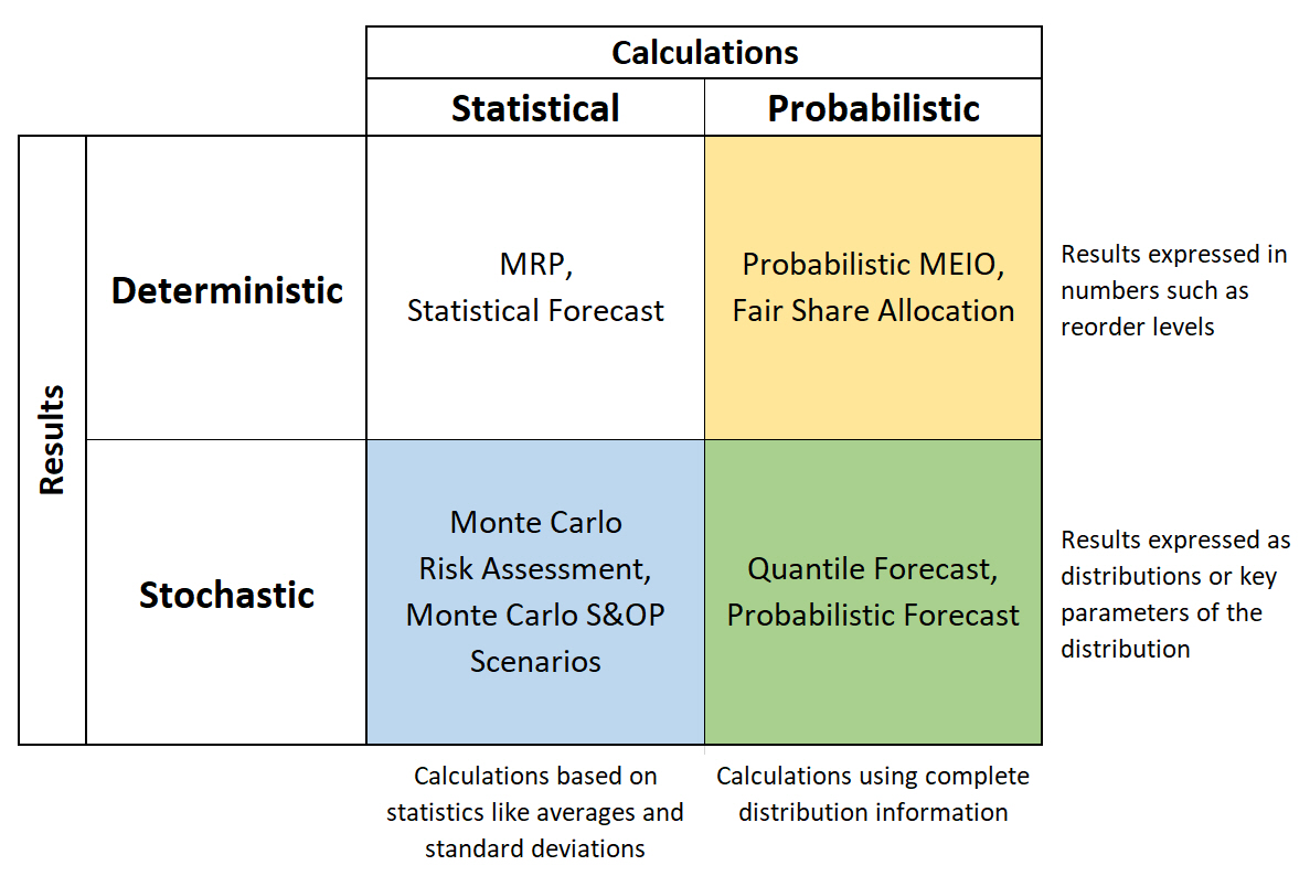
The process of obtaining both deterministic and stochastic results can be either statistical or probabilistic.
The process of preparing the input data as well as the inner calculations in a model can follow statistical or probabilistic approaches. Interestingly, the outcomes of such analysis can be either deterministic or stochastic depending on the business decision requirements. Let’s explore several examples for the possible combinations.
Statistical calculations for a deterministic result
-
MRP (material requirements planning) is a method to plan production and procurement orders considering demand, bill of materials and production lead times. This is all straightforward to calculate if the independent demand (for final product) and the lead times in all levels of supply are assumed to be deterministic. But production systems must deal with uncertainty, and statistical calculations can then help by capturing the uncertainty through calculated buffers for demand and lead times in the system.
-
Statistical forecasting is the process of fitting a curve to a set of historical data. The curve is usually chosen based on the statistical assumption that forecast residuals are independent and identically, normally distributed around zero to be unbiased. The output is a time-series of exact numbers.
Probabilistic calculations for a deterministic result
- In Probabilistic Multi-Echelon Inventory Optimization, we consider the probability distributions of the lead times and demands to optimize the overall level of inventory at different levels of supply and distribution system. The output, reorder levels or safety stock targets, are exact numbers.
- Fair Share Allocation of available inventory to customer orders when the availability is less than required. The objective is to provide each customer the same probability of stock out instead of targeting the same fill rate for different customers. The output are exact allocation quantities.
Statistical calculations for a stochastic result
- Monte Carlo Risk Assessment and Monte Carlo S&OP Scenarios return the possible behaviors based on the changes in the input parameters. The Monte Carlo simulation will repeatedly generate random but exact numbers for different scenarios following an assumed probability distribution of those problem parameters. The calculations are traditional deterministic, but the results can again be presented as empirical probability distributions where each iteration of the simulation provides one observation.
Probabilistic calculations for a stochastic result
- A quantile is the value below which a fraction of observations in a group fall. For example, a 0.75 quantile forecast should over-predict 75% of the times. Quantile forecasts are often provided for multiple quantiles simultaneously, such as 10 quantiles in the M5 forecasting competition. In such cases the output is stochastic.
- Probabilistic forecast fits distributions instead of curves. To envision this, imagine a stationary demand pattern, one where every time period has the same distribution of possible quantities. One could create a histogram for the frequency (y axis) of distinct demand quantities (x axis) similar to Figure 2 above. This histogram then displays the density of the empirical demand distribution. A proper probabilistic forecast will fit distributions even under the much more complicated situation where demand patters are not stationary. More details on probabilistic forecasting can be found in this article by Stefan De Kok.
Example in inventory control
Suppose a retail store wants to determine the optimal reorder point for a specific product to ensure adequate stock levels. The store has historical sales data for this product, but they do not know how it is distributed around the long-term patterns.
In a statistical approach, the store would assume a Gaussian (normal) distribution for the demand based on industry norms or general assumptions. Let's say the store assumes a normal distribution with a mean of 100 units and a standard deviation of 20 units for the product's demand over lead time. Using this assumption, the store calculates the reorder point based on a desired service level, such as a 95% probability of not experiencing a stockout. With the normal distribution assumption, the store might determine a reorder point of 125 units, corresponding to the mean demand plus a certain number of standard deviations to ensure sufficient inventory.
On the other hand, a probabilistic approach considers the actual data and can extract either an empirical or a parametric distribution directly from it, rather than assume one. Since the store is only learning about probabilistic methods, they choose the easier empirical approach. The store analyzes the historical sales data and constructs an empirical distribution based on the observed demand levels. It could be a histogram or a kernel density estimation, capturing the unique characteristics of the demand pattern without assuming a specific distribution shape. Using the empirical distribution, the store calculates the optimal reorder point for the desired service level. Let's say the analysis suggests a reorder point of 130 units based on the historical demand patterns.
This example highlights the distinction between statistical and probabilistic approaches in inventory control and ordering lies in the assumptions made about the distribution of demand data. While statistical approaches rely on predefined assumptions such as the normal distribution, probabilistic approaches extract the distribution directly from the data, accommodating the unique demand patterns without imposing specific assumptions. By utilizing an accurate distribution derived from the data, inventory control decisions can be enhanced in terms of accuracy and effectiveness, resulting in optimized stock levels and cost reduction.
Employing the science of probability drives better business decisions
In business decision-making, incorporating uncertainty is crucial. Different methods have been developed to handle decision-making under uncertainty, aiming to extract valuable information from data and utilize it for improved decision-making. These methods can be categorized into statistical and probabilistic frameworks.
One important distinction between these frameworks is that statistical methods rely on assumptions about the presence of specific distributions and patterns in the data. On the other hand, probabilistic methods impose minimal assumptions regarding the pattern of distribution in the data. Consequently, purpose-built probabilistic models tend to offer greater accuracy and enable better-informed business decisions.
The amount of available and high-quality data is the major criteria to choose between empirical and closed-form methods. But probabilistic methods, empirical or closed form, require no more data than their statistical equivalents, only maybe more granular. Statistical engines may allow modeling supply chains, stock markets, and airline flight control, but will be outclassed by probabilistic models in their area of focus. One last key takeaway is that the process of obtaining deterministic or stochastic results can be either statistical or probabilistic as depicted in various examples.
One of the most important applications of probabilistic models in supply chain planning is on maximizing service levels and lowering the inventory costs through probabilistic multi-echelon inventory optimization (MEIO). You can check out the Kinaxis MEIO that is integrated in RapidResponse. It optimizes the inventory across product mix, inventory tiers, and production stages, while considering physical and monetary constraints.
“First, the only certainty is that there is no certainty. Second, every decision as a consequence is a matter of weighing probabilities. Third, despite uncertainty we must decide and we must act. And lastly, we need to judge decisions not only on the results, but how those decisions were made.”
- Robert Rubin