

Forty years ago, in a freezing loading dock, the first batch of Kinaxis employees were building and assembling custom application specific integrated circuits (ASICs) for factory production planning. This was leading hardware technology for the time, and laid the groundwork for us to build our powerful CPU-based scenario planning engine.
As CPU technology improved throughout the nineties, our product shifted from custom hardware into a highly tuned CPU based scenario planning engine. When NVIDIA released the A100 GPU in 2020, it changed the landscape: this was the first GPU that we saw as powerful enough to challenge CPUs for some of our key compute workloads. Take a look here for an overview of hardware acceleration.
At the time, the mainstream perspective was that GPUs are only good at dense computations and not the sparse models common in supply chain optimization. Our prototyping showed the opposite—through hand-crafted CUDA kernels, we were able to implement a key network optimization heuristic that achieved a major speedup over the best CPU version of the algorithm. This was a highly sparse dynamic programming algorithm and the key to making it faster was to exploit the "level" structure of global supply networks. The mathematical models were very sparse, but we were able to condense them into dense echelons and exploit the density and decoupling of individual levels.
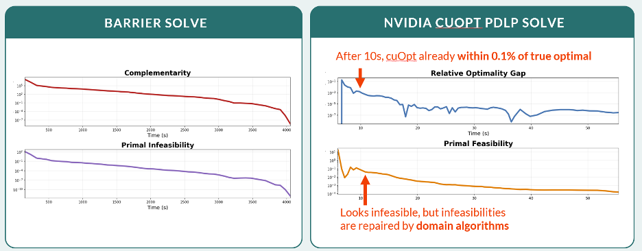
When NVIDIA released its cuOpt open-source solver and the primal-dual linear programming (PDLP) algorithm, we immediately saw the potential. It did a great job of exploiting the power of GPU compute on large, sparse matrices, so we pivoted toward using that technology rather than building and maintaining our own GPU software.
Here are the results of our most recent measurements comparing a single H100 to multiple H100s on a key subset of our internal benchmark instances. Note that this experiment isolates the PDLP phase of the solve to evaluate the scaling properties of multi-GPU PDLP:
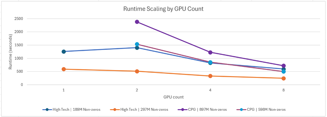
For one of Kinaxis’s largest benchmark models, moving from two GPUs to eight GPUs delivered a 3.3X speedup. While scaling properties can vary by use case and model size, this type of increase in speed is a big deal. The source optimization use case is a multi-year daily supply planning problem in the high-tech industry. The stochastic solves compute a six-month daily plan that coordinates production and distribution across a global CPG supply chain.
All this matters because these improvements don’t just make our planning solutions run faster. They enable us to tackle optimization problems that were previously too large or too computationally expensive to solve. In particular, they help us with large, globally constrained supply and production planning problems that involve daily granularity over long planning horizons.
The bigger opportunity: planning for uncertainty
The problem with the traditional way supply and production plans have been optimized is that they’re often computed with mathematical models that ignore the considerable uncertainty in supply availability, supply costs, and forecasted demand.
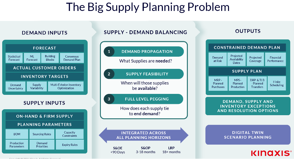
Because of this, researchers and thought leaders have put a lot of thought into stochastic optimization approaches that are capable of factoring the uncertainty into the solve itself.
Stochastic optimization: A method used to find the best or near-best solution to a problem when the data, constraints, or the search process itself involves uncertainty.
Barriers to stochastic optimization in supply planning
That said, there are some practical barriers to embracing stochastic optimization in the real world.
Barrier 1: Demand representation
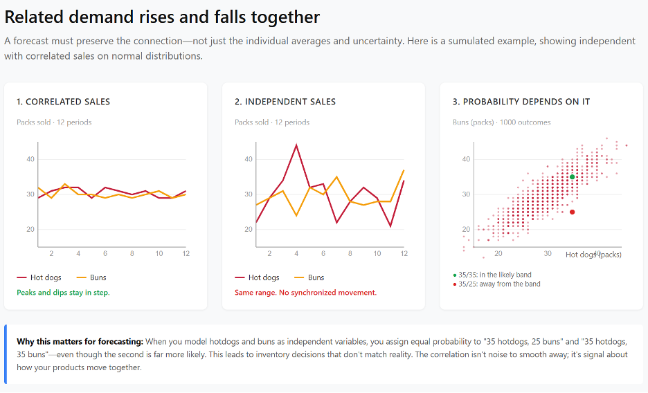
The demand forecast is a key input to the supply planning process, but it’s usually presented in a way that doesn’t capture the relationships between products.
For example, when you sell hot dogs, you’re probably also going to need to sell hot dog buns. Let’s say you usually sell about 30 packs of each, with a standard deviation of 5. A good forecasting model will capture the relationship between the items, but once that forecast gets translated into a spreadsheet database table, the relationship might fall apart. That’s how you get forecasts that tell you selling 35 packs of hot dogs and 25 hot dog buns is just as likely as selling 35 packs of each, even though the second case is much more likely.
Barrier 2: Supply plan feasibility
While a drop in demand might result in excess inventory and lost sales, it doesn’t usually upend the entire plan. However, an unexpected drop in supply can have a butterfly effect on the entire supply network, potentially making the whole plan infeasible. This asymmetry between supply and demand is one of the key difficulties in developing algorithms that account for uncertainty.
Barrier 3: Real risks are difficult to predict and quantify
Even if you have a technique that can accurately account for supply and demand variance, the main drivers of uncertainty are often abstract and extraordinarily difficult to quantify. For example, a heatwave might cause a spike in demand for air conditioners in a region that isn’t used to them. An increase in tariffs might trigger a rise in supply costs or a sudden drop in demand. A geopolitical conflict might close off a major transportation route. These potential impacts need to be quantified and included in the mathematical model.
Barrier 4: Building trust
Sometimes the plan optimized for resilience looks worse on paper than the riskier plan. If you’re trying to convince leadership to accept a plan that projects lower revenue, you need to have an explanation that goes beyond, “trust me, I’m a mathematician.” Customers need to be able to see and understand the risk and how the plan mitigates it. While detecting and fixing data quality issues matters, so does being able to explain the data.
Continuous replanning
When real disruptions occur, organizations react as quickly as they can to mitigate the impact. That means stochastic optimization models must account for the fact that planners will react and adapt over time. Otherwise, the models will always overestimate the impact of disruptions and compute plans that are heavily weighted to the worst-case scenario.
Experimenting with stochastic optimization the Kinaxis way
The approach we are experimenting with is a variation of the classic Monte Carlo simulation, where we create a large linear program model that combines hundreds or thousands of scenarios. These scenarios all start with the same fixed horizon variables, but each scenario branches into its own sub-model that represents the feasible solution space for the remainder of the horizon.
What this enables us to do is fix the decision for the first part of the horizon (e.g. the next week) that’s best across hundreds or thousands of scenarios where each scenario is being optimized independently. This has the classic min/max effect of minimizing worst case in the short term, while simultaneously optimizing for best case in the long term across each scenario.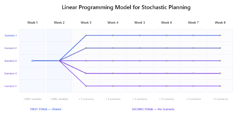
We’re exploring several ways to build on this approach:
Preserving relationships between products
We’ve been developing a foundation model for time-series forecasting, trained on NVIDIA GPUs, that can generate the baseline demand for each scenario while preserving relationships between products.
Consider the hot dog example. One scenario might project demand for 35 packs of hot dogs and 35 buns. Another might project 25 packs of each. Demand changes from one scenario to the next, but the relationship between hot dogs and buns remains intact. By generating a new forecast for each scenario directly from the model, we are able to preserve all of the non-trivial demand relationships between products.

Preserving these properties of the forecast are essential to ensure stochastic methods are optimizing for the real shape of demand uncertainty. This technique, in combination with the newly introduced multi-GPU support for NVIDIA cuOpt, enables us to accurately represent demand uncertainty by increasing the number of scenarios being simulated rather than increasing the complexity of the underlying stochastic optimization algorithm. The more complex the algorithm, the more fragile and difficult it is to apply in practice.
Making complex plans easier to explain
Our internal testing has demonstrated that with the right harness, the frontier AI models of late 2026 are capable enough to handle complex optimization explainability use cases. The Monte Carlo approach is particularly well suited to this because it gives an AI agent access to the optimal solution for thousands of sub-models, along with the risk information behind it. This is key to trust-building AI explainability.
Focusing precision where it matters most
We don’t need a high-fidelity solution for thousands of scenarios. In fact, we don’t want one. Wasting compute capacity on high precision solutions when low precision will get the job done is like having a critical bottleneck machine sitting idle on a factory floor.
If the model supports a weekly planning process, then the most important question is: “What decisions do we need to make this week?”
Those near-term decisions require a high-fidelity answer. Decisions in the weeks ahead don’t matter to this process, because the model will run again next week using the latest information to produce a high precision plan for that week. What matters today is understanding how those longer-term possibilities should influence the actions planners take now.
This all plays to the strengths of the PDLP algorithm, which has the unique ability to quickly approach a near-optimal solution to extremely large linear programs. The algorithm itself was designed to take advantage of massively parallel hardware and NVIDIA cuOpt has an efficient implementation that delivers on this potential.
Curious about how it works? Test it yourself
If you would like to measure the impact of multi-GPU optimization on your large LP models for yourself, cuOpt is very easy to test and run locally. To do a single-GPU PDLP solve, you can run the following command, which will download the latest cuOpt version from Docker Hub and solve a sample MPS file file with it:
> docker run -it --rm --gpus all -v $PWD/sample.mps:/data/sample.mps nvidia/cuopt:latest-cu12 cuopt_cli --method 1 --num-gpus 2 /data/sample.mps
If you would like to experiment with the new multi-GPU capability, just increase the “—num-gpus” parameter to the number of GPUs you would like to use and look for the log line “Solving with distributed PDLP on <N> GPUs.”
Kinaxis, NVIDIA, and the road ahead
Kinaxis is excited to continue working closely with NVIDIA on the cutting edge of mathematical optimization and AI. And we’re always on the look-out for co-innovation partners. If you’re in the business of managing complex supply chains and are interested in co-innovation with us on these topics, please reach out to innovation@kinaxis.com