
Here on the development team, we are big fans of iterative development for our software, for our ML models and especially for our office table tennis ranking system! In the past, our team wrote about Building A Table Tennis Ranking Model using the Bradley-Terry model and Google sheets. The model gives a single rating for each player (not unlike the Elo rating system in Chess). One drawback of this model is that it has no measure of “confidence”. For example, a new player could have a single lucky game against the reigning champion and suddenly soar to the top of the rankings, but should we be that confident in their ranking? Enter Bayesian Hierarchical Modelling.
Hierarchical Bayesian models
Many of the parametric models you know and love (such as linear regression or MLPs), use a maximum likelihood estimate (MLE) or maximum a posterior (MAP) to estimate the parameters
where
Bayesian hierarchical modelling takes a slightly different philosophical approach. Every parameter of interest in the model is a random variable with its own distribution. This means we can ask our usual questions of a random variable such as: what’s the mean? median? standard deviation?
Bayesian modelling always starts off with a statement of Bayes theorem describing the relationship between the parameters of interest and the data:
The likelihood and prior (aka regularizer) from our MAP estimate above are included there along with a constant factor in the denominator. The MAP estimate attempts to find a point-estimate that maximizes the RHS of Equation 2, while a full Bayesian analysis attempts to find the distribution specified by
Once we have a distribution for each parameter, we can generate the credible interval (or region for multi-variate distributions) which involves finding an interval
A Bayesian ranking model
To define our Bayesian hierarchical model, we need to specify the likelihood and prior functions from Equation 2 (the marginal likelihood is a constant so we don’t need to specify it). We’re going to follow the Bradley-Terry model, where we assume that the probability of player
where
In this case, we’re assuming that each player’s rating has equal probability of being any possible rating in
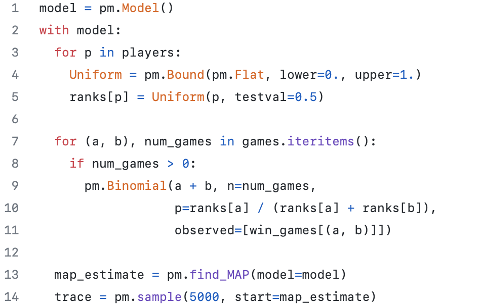
In recent years, Bayesian statistical packages have come a long way. There are simple interfaces with heavily optimized engines to fit Bayesian models. The most popular Bayesian statistics package is Stan, but we ended up using PyMC3 because we like the native Python interface. For a simple model like this, there’s not much difference in performance so usability is the main concern.
The nice thing about these packages is that you can take Equation 4 and basically translate it directly, here’s a code snippet of our model in PyMC3:
The official Rubikloud/Kinaxis table tennis rankings V2
We're happy to announce that we've since moved on to V2 of our table tennis rankings. To simplify the UI, instead of plotting each individual’s distribution, we simply show each person’s 50% credible interval centered on the MAP estimate:
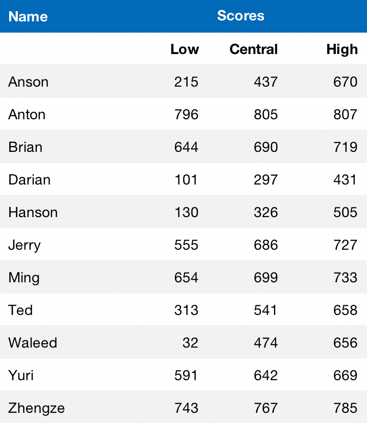
The scores are put on a logarithmic scale and scaled from 1 to 1000. Visually it looks like this:
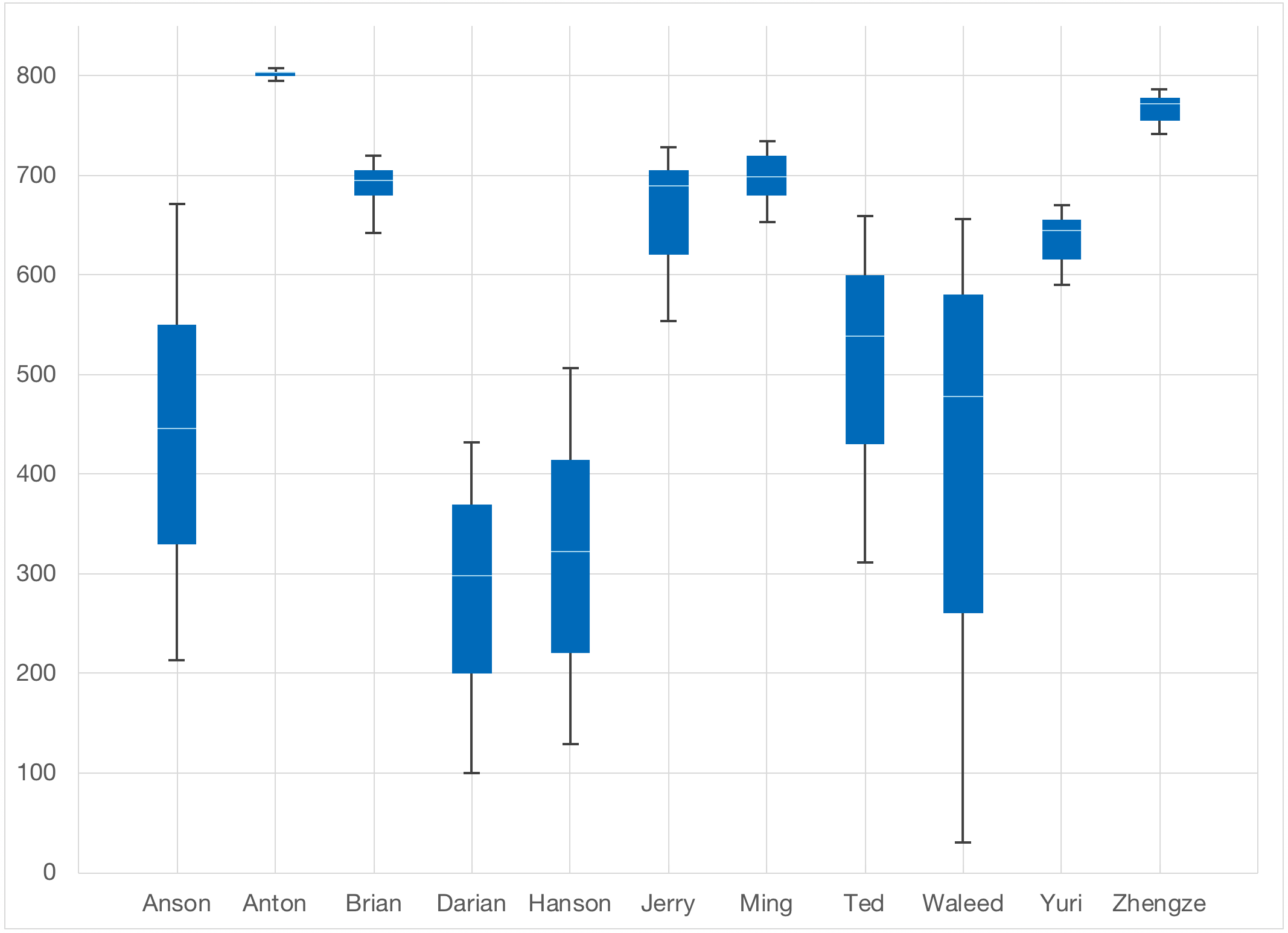
As you can see from this past example, some players had a very wide range while others had a very tight range. This shows the “confidence” the model has in the rating. Since this time, the changes were well-received, with players consistently showing more interest in trying to move up the rankings.
Editor's note: This blog is part of a series originally published on Rubikloud's blog, "kernel." Kinaxis acquired Rubikloud in 2020.
Leave a Reply